tomoxide
A Rust tomographic reconstruction toolkit — the algorithmic breadth of tomopy fused with the GPU-accelerated streaming reconstruction of tomocupy, behind a single tri-backend abstraction: CPU · CUDA · wgpu (Metal / Vulkan / DX12).



All three backends reconstruct real beamline datasets. The CPU backend
ports tomopy's analytic (fbp, gridrec, fourierrec, lprec, linerec)
and iterative (sirt, mlem, osem, ospml, pml, tv, grad, tikh,
art, bart) families; the CUDA backend ports tomocupy's device-resident
streaming kernels (multi-GPU, fp16, laminography, and the full iterative suite
on-device); the wgpu backend runs a portable subset with no NVIDIA toolkit.
Why
| tomopy | tomocupy | tomoxide | |
|---|---|---|---|
| Language | Python + C (libtomo) | Python + CUDA (CuPy) | Rust |
| Algorithm breadth | ✅ broad | ⚠️ fourierrec/lprec/linerec | ✅ union of both |
| GPU acceleration | ⚠️ partial | ✅ CUDA streaming | ✅ CUDA + portable wgpu |
| Streaming / on-the-fly | ❌ | ✅ chunked, double-buffered | ✅ (port of rec_steps) |
| Memory safety | C | CUDA/C++ | ✅ Rust |
| Runs without an NVIDIA GPU | ✅ (CPU) | ❌ | ✅ (CPU or Metal via wgpu) |
Install
The library and CLI are published on crates.io:
# Library — add to a Rust project
cargo add tomoxide

# Command-line reconstruction tool
cargo install tomoxide-cli
The default build is pure-CPU with no system dependencies. Opt into the GPU backends and extras with cargo features:
# CUDA backend (needs the CUDA toolkit / nvcc)
cargo add tomoxide --features cuda

# Portable GPU backend (wgpu: Metal / Vulkan / DX12)
cargo add tomoxide --features gpu-wgpu
Other features: config (TOML recipes, shared by the CLI and GUI),
beam-hardening (xraylib), sift-center (pure-Rust SIFT center finding).
Workspace layout
Two published crates plus a desktop GUI that lives in the repo but outside the Cargo workspace:
crates/
  tomoxide       library: data model, geometry, the Backend trait, all three
                 backends, reconstruction, preprocessing, I/O, simulation,
                 and the high-level streaming pipelines
  tomoxide-cli   command-line front-end (init / status / recon / recon_steps / tune_chunk)
  tomoxide-gui   desktop app (rsplot / egui + wgpu) — not published to crates.io
This book
- Architecture — the
Backendtrait, the tri-backend design, threading, and the streaming pipelines. - Algorithms — the analytic and iterative reconstruction families and their filters, geometry, and conventions.
- Benchmarks — cross-backend timing and accuracy, including FBP-vs-iterative comparisons against known-truth phantoms.
- Desktop GUI — the six-mode
tomoxide-gui(Data / Tune / Center / Run / Output / Live) and its offline + live-streaming design. - Porting & tomocupy parity — how the CUDA/CPU backends were ported and validated against the upstream tomopy / tomocupy originals.
The full API reference is on docs.rs/tomoxide.
License
See the repository for license details.
tomoxide — Architecture
This document defines the data model, the tri-backend abstraction, the reconstruction taxonomy, and the streaming pipeline. It is the contract that every module stub in the workspace is written against.
The two upstream projects map onto tomoxide as two complementary halves:
- tomopy contributes algorithmic breadth on the CPU (
libtomo): gridrec, FBP, and the iterative family (ART, BART, SIRT, MLEM, OSEM, OSPML/PML, TV, TIKH, GRAD, vector), plus a rich preprocessing/misc library. - tomocupy contributes GPU streaming throughput (CUDA): Fourier-based
reconstruction (
fourierrec), log-polar (lprec), direct line integration (linerec), laminography (USFFT), and a chunked, double-buffered, multi-stream pipeline for out-of-core datasets.
tomoxide unifies them: one data model, one set of capability traits, three interchangeable backends.
1. Data model (tomoxide-core::data)
All bulk arrays are f32 by default (f16 is a first-class option on the GPU
backends, mirroring tomocupy's --dtype float16). Arrays are 3-D and carry an
explicit axis layout so we never silently transpose:
| Type | Axes (slowest→fastest) | tomopy/tomocupy name |
|---|---|---|
Projections | [angle, row, col] = (dt,dy,dx) | "projection order" (default) |
Sinogram | [row, angle, col] = (dy,dt,dx) | "sinogram order" (sinogram_order=True) |
Volume | [z(row), y, x] | reconstructed object |
Slice2D | [y, x] | one reconstructed slice |
Layout::{Projection, Sinogram} is tracked at the type level; conversion is an
explicit swap_axes(0,1) (the same operation tomopy performs internally). The
column axis x/col is the detector width; row/y indexes the slice (the
reconstruction is independent and parallel per row for parallel-beam geometry).
Auxiliary fields (the DXchange triple):
data— projections, the array above.flat/white— flat-field (open-beam) frames[nflat, row, col].dark— dark-field frames[ndark, row, col].theta— projection angles,[angle], radians.
Geometry (tomoxide-core::geometry)
Geometry {
    angles: Angles,          // radians, length = n_proj
    center: Center,          // rotation axis: scalar or per-row
    beam:   Beam,            // Parallel | Cone { source_dist } | Laminography { tilt }
    detector: Detector { width, height, pixel_size }
}
Center is Scalar(f32) or PerRow(Vec<f32>) because tomopy accepts a center
array (one per slice) and tomocupy searches it per chunk. Laminography carries
the pitch angle phi that tomocupy's linerec/USFFT kernels take.
2. Backend abstraction (tomoxide-core::backend)
The central design decision. Algorithms are written once, against capability traits, and dispatched to whichever backend the caller selected.
2.1 Device & buffers
#![allow(unused)]
fn main() {
pub trait Backend: Send + Sync {
    fn name(&self) -> &'static str;
    fn device(&self) -> DeviceKind;          // Cpu | Cuda | Wgpu
    fn supports(&self, dt: Dtype) -> bool;   // e.g. CPU has no f16 FFT
}

pub trait DeviceBuffer<T: Element> {
    fn len(&self) -> usize;
    fn is_empty(&self) -> bool { self.len() == 0 }
    fn copy_from_host(&mut self, src: &[T]) -> Result<()>;
    fn copy_to_host(&self, dst: &mut [T]) -> Result<()>;
}
}
A Buffer<T> lives on the device. On the CPU backend it wraps an
ndarray/Vec; on CUDA it wraps a device pointer + stream; on wgpu it wraps a
wgpu::Buffer. Host↔device copies are explicit, matching tomocupy's
pinned-memory staging.
2.2 Capability traits
Each numerical primitive the pipeline needs is one trait. A backend implements
the subset it supports; missing ones return Error::NotImplemented.
| Trait | Method(s) | Upstream origin |
|---|---|---|
Fft | fft_1d, ifft_1d, fft_2d, ifft_2d (batched, R2C/C2R) | cuFFT (tomocupy cfunc_fft2d) / rustfft (CPU) |
FbpFilter | make_filter(name, n), apply(sino, filter, center) | tomocupy cfunc_filter; tomopy fbp.c |
FilteredBackproject | backproject(sino, geom, out) | fourierrec / lprec / linerec / gridrec.c |
ForwardProject | project(volume, geom, out) | tomopy project.c |
RayProject | ray_rows(geom, n) (sparse single-ray rows of R) | tomopy art.c, bart.c (row-action Kaczmarz) |
Elementwise | darkflat, minus_log, clip, axpy | tomocupy proc_functions; tomopy normalize |
RankFilter | median3d, remove_outlier | tomopy median_filt3d.c |
Algorithms in tomoxide-recon/tomoxide-prep take &dyn Backend (plus the
capability trait objects the backend exposes) and never name a concrete device.
This is what lets the same fbp() run on CPU, CUDA, or Metal.
2.3 The three backends
                 ┌──────────────────────── tomoxide-core ───────────────────────┐
                 │   data · geometry · Dtype · Error ·  capability traits        │
                 └───────────────┬───────────────┬───────────────┬──────────────┘
                                 │               │               │
                 ┌───────────────▼──┐  ┌─────────▼─────────┐  ┌──▼───────────────┐
                 │  tomoxide-cpu    │  │  tomoxide-cuda    │  │  tomoxide-wgpu   │
                 │  ndarray+rayon   │  │  FFI → *.cu/nvcc  │  │  WGSL compute    │
                 │  rustfft         │  │  cuFFT, cuda      │  │  Metal/Vulkan    │
                 │  always builds   │  │  feature = "cuda" │  │  feat=`gpu-wgpu` │
                 └──────────────────┘  └───────────────────┘  └──────────────────┘
- CPU (
tomoxide-cpu): the parity target forlibtomo. Pure Rust (ndarray,rayon,rustfft). Always compiles; the reference for tests. - CUDA (
tomoxide-cuda): re-uses tomocupy's battle-tested.cukernels. A thinextern "C"shim wraps the SWIG-exposedcfunc_*C++ classes; abuild.rsinvokesnvcconly when thecudafeature is set, so a machine without a CUDA toolkit still builds the rest of the workspace. The kernel directory is given byTOMOXIDE_CUDA_KERNELS(defaults to a vendoredcuda/copy). See §4. - wgpu (
tomoxide-wgpu): a portable compute backend (Metal on macOS, Vulkan/DX12/GL elsewhere) so the GPU path runs on hardware tomocupy can't target. Kernels are WGSL ports of the CUDA kernels. Optional (gpu-wgpu) becausewgpuis a heavy dependency; the default workspace build skips it.
2.4 Backend selection
tomoxide::Engine::auto() probes at runtime in order: CUDA (if compiled and a
device is present) → wgpu (if compiled and an adapter is present) → CPU. The
CLI exposes --backend {auto,cpu,cuda,wgpu}.
3. Reconstruction taxonomy (tomoxide-recon)
Two families, dispatched by a single recon(sino, geom, Algorithm, backend).
3.1 Analytic / direct (one pass: filter → backproject)
| Algorithm | Backend(s) | Upstream |
|---|---|---|
Fbp | CPU, CUDA, wgpu | tomopy fbp.c; filter is shared with gridrec |
Gridrec | CPU | tomopy gridrec.c (Fourier grid + convolution) |
Fourierrec | CUDA, wgpu | tomocupy cfunc_fourierrec (USFFT, exponential interpolation) |
Lprec | CUDA, wgpu | tomocupy cfunc_lprec (log-polar) |
Linerec | CUDA, wgpu | tomocupy cfunc_linerec (direct line integral; laminography) |
The FBP filter kernel (ramp, shepp, cosine, cosine2, hamming, hann,
parzen, none) is shared across CPU and GPU — both tomopy and tomocupy expose
the same set.
3.2 Iterative (project ↔ backproject loop)
| Algorithm | params | Upstream |
|---|---|---|
Art | num_iter | tomopy art.c |
Bart | num_iter, num_block, ind_block | tomopy bart.c |
Sirt | num_iter | tomopy sirt.c |
Mlem | num_iter | tomopy mlem.c |
Osem | num_iter, num_block, ind_block | tomopy osem.c |
OspmlHybrid | num_iter, reg_par, num_block, ind_block | tomopy ospml_hybrid.c |
OspmlQuad | num_iter, reg_par, num_block, ind_block | tomopy ospml_quad.c |
PmlHybrid | num_iter, reg_par | tomopy pml_hybrid.c |
PmlQuad | num_iter, reg_par | tomopy pml_quad.c |
Tv | num_iter, reg_par | tomopy tv.c |
Grad | num_iter, reg_par | tomopy grad.c |
Tikh | num_iter, reg_data, reg_par | tomopy tikh.c |
Cgls | num_iter | standard CGLS (Björck); parity-checked vs ASTRA CglsAlgorithm |
Vector{,2,3} | num_iter, axis… | tomopy vector.c |
Most iterative solvers reduce to ForwardProject + FilteredBackproject
(unfiltered backproject) capability calls, so the same solver loop runs on any
backend that provides those two primitives. The row-action methods (Art,
Bart) are the exception: they update the reconstruction one ray at a time, so
they use the RayProject (single-ray) capability instead.
For each method's strengths, use cases, and a selection guide (plus the
device-resident GPU benchmark), see ALGORITHMS.md.
3.3 Center finding (tomoxide-recon::center)
find_center (entropy), find_center_vo (Vo coarse+fine, the workhorse),
find_center_pc (phase correlation), plus tomocupy's SIFT/AI variants
(find_center_sift, find_center_ai) behind feature flags.
4. CUDA FFI boundary (tomoxide-cuda)
tomocupy exposes C++ classes through SWIG; we cannot link SWIG's Python module,
so tomoxide adds a thin C-ABI shim (cuda/shim.cpp) that wraps each
cfunc_* class in extern "C" create/destroy/call functions:
// generated shim, one set per kernel class
void*  tomoxide_fourierrec_new(size_t nproj, size_t nz, size_t n, const float* theta);
void   tomoxide_fourierrec_backproject(void* h, void* f, const void* g, void* stream);
void   tomoxide_fourierrec_free(void* h);
Rust side (ffi.rs) declares these as extern "C" and CudaBackend owns the
opaque handles. build.rs:
- runs only if
cfg!(feature = "cuda")(guarded byCARGO_FEATURE_CUDA); - resolves the kernel dir from
$TOMOXIDE_CUDA_KERNELS(default./cuda); - shells out to
nvccto compilecfunc_*.cu+shim.cppinto a static lib for the gencode arches in$TOMOXIDE_CUDA_ARCH(default75;80;86;89;90); - emits
cargo:rustc-link-lib=cudart,cufft, and the shim archive.
Without the feature, build.rs is a no-op and CudaBackend::new() returns
Error::BackendUnavailable.
Buffer pointers and CUDA stream handles cross the boundary as opaque void*
(tomocupy passes them as size_t); Rust treats them as *mut c_void. The
f16 variants correspond to tomocupy's *fp16 classes, selected by Dtype.
4.1 CUDA analytic output convention (vs CPU/wgpu)
The vendored tomocupy back-projection / Fourier kernels originally carried
tomocupy's own output convention (y-flipped, 4/nproj back-projection, a ½
filter gain), which differed from the CPU/wgpu (tomopy) path. A cross-backend
convention unification brought the CUDA analytic output onto the CPU/tomopy
convention, so for the same sinogram, geometry, and centre a CUDA analytic
reconstruction now matches the CPU/wgpu output in both orientation and scale:
| algorithm | image orientation | amplitude scale (cuda / cpu) |
|---|---|---|
fbp, linerec | same as CPU | ≈ 1 (back-projection dθ weight 4/nproj → π/nproj at the analytic call sites, filter ½ removed) |
fourierrec | same as CPU | ≈ 1 (filter ½ removed, unnormalized cuFFT inverse normalized by (2n)²) |
lprec | same as CPU | ≈ 1 (filter ½ removed; log-polar back-projection already matched the CPU port) |
gridrec | same as CPU | 1 (backend-agnostic recon::gridrec over the Fft capability; never used build_filter_w) |
What the unification changed (the CPU/wgpu backends port tomopy, the CUDA backend ports tomocupy, and the unification target is tomopy):
- Orientation — the tomocupy y-flip was removed from
cfunc_linerec(storage-index un-flip) andcfunc_fourierrec(a clean output-row flip indivphi), so CUDA emits the CPU/tomopy handedness. Both back- and forward-projectors were flipped together, so they remain a discrete transpose. - Filter amplitude — the CUDA-only
½inbuild_filter_w(tomocupy's net FBP gain) was dropped; the gain is now1/pad, matching tomopy. - Back-projection scale —
cfunc_linerec's baked-inc = 4/nproj(tomocupy) became a caller-supplied gain: the analytic FBP call sites pass theπ/nprojangular-quadrature dθ weight (tomopy scale), while the iterative solvers pass1.0— the back-projector itself is the pure adjointWᵀof the unweighted line-integral forward projectorWon every backend, so a converged iterative solve yields the physical μ (pinned absolutely bytests/iterative_amplitude.rs). - fourierrec normalization — cuFFT does not normalize its inverse transform
and
plan2dis(2n)², so the CUDA fourierrec ran(2n)²× hot;divphinow divides by(2n)²to match the CPU's normalized inverse FFT.
Absolute scale = physical μ. Beyond cuda/cpu agreement, the analytic output
is anchored to an absolute scale: the make_fbp_filter base ramp is the physical
|ω| inversion filter (peak 0.5 at Nyquist), not tomopy/tomocupy's doubled
ramp (peak 1), and recon::gridrec's ramp_scale is π/nang with no matching
empirical ×2. So every analytic method reconstructs the attenuation μ per
pixel-unit rather than 2×μ — the same scale the iterative solvers converge
to, which makes fbp→iterative warm-starts scale-consistent. Pinned by tests/analytic_amplitude.rs (a unit
disk reconstructs to core mean ≈ 1.0). This is a deliberate departure from both
upstreams, whose absolute analytic amplitude is itself convention-dependent
(tomopy gridrec ≈ 1.16×μ via an empirical winv fudge; tomocupy ≈ 4/π×μ).
Ramp shape (the remaining cuda/cpu residual). The base ramp still differs per
backend: CPU/wgpu build tomopy's plain linear ramp (k/pad), CUDA builds
tomocupy's degree-12 _wint quadrature ramp (pad·wint(t)), selected via
backend::RampShape (Linear for CPU/wgpu, Wint for CUDA and for
recon::lamino on every backend) in the single shared make_fbp_filter. This leaves
a deterministic ~1.6% amplitude residual on the unified paths (the measured
cuda/cpu scale is ≈1.016, not exactly 1); Pearson stays ≈1.0 because the shape
difference is small and smooth. This is a shape convention, not a numerical error.
Laminography is excluded from the scale unification — but not from the
orientation one. The CUDA lamino path (cfunc_linerec tilted back-projector) and
the CPU lamino path (recon::lamino, a USFFT algorithm) are different
reconstruction algorithms, so their amplitudes are not comparable and are
not unified.
Their handedness and sign, however, are shared with everything else:
- No y-flip on either side. The CUDA lamino kernel lost tomocupy's
(n−1−ty)write together with the rest ofcfunc_linerec(Phase 1). The USFFT pair (recon::lamino,lam_divker2d_adj_ker) kept tomocupy'sn1−ty−1divker row, which tomocupy added to match its own y-flipped linerec, until it too was dropped. Alamino_project → laminoround trip cannot see a flip both sides share, sotests/lamino_orientation.rspins the CPU pair to the parallel projector at zero tilt, andcuda_lamino_fourierrec.rspins Fourierrec and Linerec to the volume of a 20° scan. - Positive attenuation for dense material on both, since the Fourier-lamino
sign fix dropped tomocupy's
irfftshiftcglobal−1fromrecon::lamino.
No cuda/cpu lamino ratio is quoted here. An earlier revision of this section
gave one; it is not reproducible, and the quantity is not meaningful to begin with
— fed one shared sinogram the two reconstructions correlate at only r ≈ 0.3, so
a least-squares scale between them summarises nothing. Each lamino path is
validated against its own reference (CUDA vs tomocupy, CPU vs wgpu) rather than
against each other. Consumers must not assume CUDA and CPU laminography agree in
absolute amplitude.
The cross-backend regression test tests/cuda_cpu_convention_parity.rs pins both
the orientation and the cuda/cpu ≈ 1 scale (|Δ| < 5%) for fbp/linerec/fourierrec/
lprec, so any re-appearance of a per-algorithm convention scale — or any other CUDA
divergence — fails there rather than hiding behind a scale-invariant metric.
5. Streaming pipeline (tomoxide::pipeline)
Direct port of tomocupy's two execution modes, layered over the backend traits.
5.1 Full, in-memory (rec.py::GPURec)
For datasets that fit in device memory. Reads everything, preprocesses, reconstructs, writes.
5.2 Chunked / streaming (rec_steps.py::GPURecSteps) — the throughput path
Out-of-core. Two chunking axes and a 3-stage software pipeline that overlaps disk I/O, host↔device transfer, and compute:
 read thread        stream 1 (H2D)      stream 2 (compute)     stream 3 (D2H)     write threads
 ───────────        ──────────────      ──────────────────     ──────────────     ─────────────
 HDF chunk ──▶ pinned[k%2] ──▶ gpu[k%2] ─▶ proc_sino           ─▶ rec_gpu ─▶ pinned ─▶ TIFF/HDF/zarr
 (max_read_threads)            (set)        proc_proj             (.get)
                                            fbp_filter_center
                                            backprojection
- Sinogram chunking (
proc_sino_parallel):nczrows per chunk overz; dark/flat correction, outlier removal (dezinger), stripe removal, minus-log, beam hardening. - Projection chunking (
proc_proj_parallel):ncprojangles per chunk; phase retrieval, beam hardening, projection rotation, double-FOV handling. - Double buffering: index
k%2ping-pongs pinned/device buffers so stage k+1 uploads while stage k computes and stage k-1 downloads.
In tomoxide this is expressed with backend-agnostic buffers and Rust threads
(std::thread + channels) for the read/write pools; the per-backend "stream"
is an associated Stream type (a real cudaStream_t, a wgpu::Queue
submission, or — on CPU — a rayon scope). The orchestration code is written
once.
The try / try_lamino modes (single-slice reconstruction across a sweep of
candidate centers / laminography angles) reuse the same chunk machinery with a
shift array, feeding find_center.
6. Crate dependency graph
tomoxide-core  ◀── everything (types, traits, errors)
      ▲
      ├── tomoxide-cpu      (impl traits, ndarray/rayon/rustfft)
      ├── tomoxide-cuda     (impl traits, FFI; feature "cuda")
      ├── tomoxide-wgpu     (impl traits, WGSL; feature "gpu-wgpu")
      ├── tomoxide-recon ──▶ depends on core only (backend-agnostic algorithms)
      ├── tomoxide-prep  ──▶ depends on core only
      ├── tomoxide-io
      └── tomoxide-sim
                 ▲
   tomoxide (umbrella) ── re-exports all of the above, owns Engine + pipeline
                 ▲
        tomoxide-cli ── clap front-end (init/recon/recon_steps/status)
recon/prep deliberately depend on core only, not on any backend crate —
they receive a backend through trait objects. Backend crates are wired together
in the tomoxide umbrella, which is the only place that knows all three exist.
tomoxide — Iterative Algorithm Guide
Practical companion to ARCHITECTURE.md §3.2,
which lists each iterative algorithm's parameters and tomopy upstream. This
document covers what each method is good at and when to reach for it,
how to chain methods (warm-start), plus the measured GPU behaviour of the
device-resident suite.
Scope of the claims. The "strengths / use cases" below are the design properties of each algorithm (as defined by tomopy and the reconstruction literature). What tomoxide has verified empirically is: (a) every CUDA device-resident method reproduces the per-iteration CUDA path at Pearson r = 1.000000, and (b) the wall-clock numbers in §5. A per-sample reconstruction-quality comparison across methods (on one real dataset) lives in
BENCHMARKS.md— consult it for measured quality/filter/iteration behaviour, then validate on your own data.
1. Families at a glance
| Family | Members | Core update | Positivity |
|---|---|---|---|
| Row-action (Kaczmarz) | Art, Bart | one ray (ART) / one block (BART) at a time | no |
| Least-squares / SIRT | Sirt, Grad, Tikh, Cgls | gradient / conjugate-gradient of ‖Ax − b‖² (+ regularizer) | no |
| Statistical EM (Poisson) | Mlem, Osem | multiplicative x ∘ Aᵀ(b ⊘ Ax) ⊘ Aᵀ(1) | yes (by construction) |
| Penalized-ML (De Pierro) | PmlQuad, PmlHybrid, OspmlQuad, OspmlHybrid | EM step + 8-neighbour smoothness prior | yes |
| Total variation | Tv | Chambolle–Pock primal–dual on ‖Ax−b‖² + λ‖∇x‖₁ | no |
A = forward projector, Aᵀ = back-projector, b = measured sinogram.
2. Per-algorithm reference
Row-action — Art, Bart
- ART projects the reconstruction onto each ray's hyperplane sequentially,
updating immediately so the next ray sees the change.
- Strengths: fast early convergence in few iterations; simple; needs no parameter; works when angles are few or unevenly sampled.
- Use for: sparse / limited-angle data, quick previews.
- BART is block (ordered-subset) ART: within a subset every ray reads the
same reconstruction, corrections accumulate, and the block is applied once.
- Strengths: averages out per-ray noise sensitivity that plain ART has; more parallel.
- Use for: the ART situations above when data is noisier.
- Cost note: in tomoxide ART/BART are pure host computation (geometry-only
RayProjectrows; the Kaczmarz sweep is inherently sequential). CUDA output is bit-identical to CPU, and there is essentially no GPU speed-up (~1×).
Least-squares & SIRT — Sirt, Grad, Tikh, Cgls
- SIRT — parameter-free, convergent
x ← x + C∘Aᵀ(R∘(b − Ax))withR = 1/A(1),C = 1/Aᵀ(1).- Strengths: very stable and robust, no tuning, gentle on noise.
- Use for: the safe default baseline; noisy data; "just give me something reliable".
- GRAD — explicit least-squares gradient descent (with a Barzilai–Borwein
step by default).
- Strengths: flexible step control; explicit
‖Ax − b‖²minimization. - Caveat: unregularized GRAD + BB is run-to-run unstable — there is no contraction, so the atomic-add nondeterminism in forward/back-projection drives divergent BB step sizes. Use a fixed step, or prefer TIKH, if you need reproducibility. (This is why the parity test fixes the GRAD step and uses BB only for TIKH.)
- Strengths: flexible step control; explicit
- TIKH — GRAD plus a Tikhonov ridge
‖x − prior‖²(reg_datasupplies the optional prior volume).- Strengths: the ridge contracts → stable (BB step is safe); can fold in a prior/reference volume.
- Use for: when you have a prior volume, or when GRAD is too unstable.
- CGLS — conjugate-gradient least squares (the standard algorithm, Björck;
its recurrence cross-checked against ASTRA's
CglsAlgorithm, implemented independently — ASTRA is GPL-3.0, no ASTRA code is used): a Krylov solver of the same‖Ax − b‖²normal equations as GRAD/SIRT, but with the optimal step and conjugate search directions, so it reaches a given residual in far fewer iterations (≈4–30× vs SIRT here). Parameter-free; per-slice scalars; CUDA device-resident.- Strengths: fastest convergence of the least-squares family; no tuning.
- Caveat: no built-in regularization — on ill-posed (sparse/noisy) data it semi-converges quickly, so it needs early stopping (peak quality often at ~10 iterations, then it fits sparse-view/noise artifacts). Being a Krylov method it is also more float-order sensitive than the contractive solvers (device vs host agree to ~1e-2 relative, Pearson ≈ 1, not the ~1e-8 of SIRT).
- Use for: well-posed / densely-sampled data, or a fast few-iteration solve; pair with early stopping on sparse/noisy data. For noisy data prefer TV.
Statistical EM — Mlem, Osem
- MLEM — multiplicative EM update; the maximum-likelihood estimator for
Poisson-distributed counts.
- Strengths: optimal noise model for low-dose / low-count data; output is always non-negative by construction.
- Use for: low-dose CT, low photon counts, emission-style data.
- OSEM — MLEM restricted to ordered angle subsets (
num_block); one outer iteration doesnum_blocksub-updates.- Strengths: ~
num_block× faster early convergence — reaches MLEM quality in far fewer outer iterations. It is the practical replacement for MLEM. - Use for: whenever MLEM is appropriate but you want speed. Also the biggest GPU device-residency win (many subset back-projections per iteration).
- Strengths: ~
Penalized-ML — PmlQuad, PmlHybrid, OspmlQuad, OspmlHybrid
EM data term plus a De Pierro 8-neighbour smoothness prior (reg_par[0] =
strength; reg = 0 reduces exactly to MLEM/OSEM). Ospml* add ordered subsets
on top (like OSEM); Pml* are the single-block case.
- quad (
PmlQuad,OspmlQuad) — quadratic prior (γ = 1).- Strengths: smooths noise strongly and uniformly.
- Use for: low-dose data where MLEM/OSEM is too noisy.
- hybrid (
PmlHybrid,OspmlHybrid) — edge-preserving priorγ = 1/(1 + |Δ|/δ),δ = reg_par[1].- Strengths: smooths flat regions while preserving edges across large jumps.
- Use for: low-dose + samples where sharp boundaries matter.
- Cost note:
Ospml*show the largest device-residency speed-up in tomoxide (per-iteration stencil + subset back-projections are all kept on the GPU) — see §5.
Total variation — Tv
Chambolle–Pock primal–dual on ‖Ax − b‖² + λ‖∇x‖₁ (λ = reg_par[0]).
- Strengths: piecewise-smooth reconstruction with sharp edges; strong on sparse-view / limited-angle data; suppresses streak/staircase artefacts in homogeneous regions.
- Use for: few-angle acquisitions, samples with large uniform regions and distinct boundaries (materials, contrast-enhanced).
3. Selection guide
| If you… | Reach for |
|---|---|
| are unsure / want a safe, tuning-free baseline | SIRT |
| have low-dose / low-count (Poisson) data | OSEM (MLEM quality, faster) |
| have low-dose data that comes out too noisy | OSPML-quad, or OSPML-hybrid to keep edges |
| have few / limited angles | TV (or ART/BART) |
| have a prior volume, or GRAD is unstable | TIKH |
| want maximum GPU throughput | OSEM / OSPML (largest device-residency gain) |
| need reproducible least-squares | SIRT or TIKH (avoid unregularized GRAD+BB) |
| want faster convergence, or a rough pass then a polish | chain an analytic seed into an iterative method (see §4) |
4. Chaining (warm-start)
An iterative reconstruction does not have to start from a blank (or flat)
volume — it can be warm-started from another reconstruction's output through
ReconParams.init. This is the tomography analogue of ptychography's engine
chaining (DM/RAAR → ML): run a fast method to get a good global estimate, then
hand it to a second method to refine.
Two motivations, both about quality per iteration, not escaping local minima (tomographic least-squares is largely convex):
- Convergence speed. An analytic seed already carries the low-frequency structure that an iterative-from-zero solver spends many iterations building up, so the iterative pass starts far closer to the answer.
- Regularizer polish. A cheap rough reconstruction followed by a regularizing method (TV, PML) cleans up noise/streaks the first pass left.
Producers vs. consumers
- Seed producers — any full-volume reconstruction. The analytic / direct
methods
Fbp,Gridrec,Fourierrec,Lprec,Linerec(whichever your backend provides) are the natural first stage: one fast pass, no tuning. The output of any iterative method can equally seed the next. - Seed consumers (
ReconParams.init) — every iterative method except the row-action pairArt/Bart, which sweep single rays and have no whole-volume iterate to seed (they reject a non-Noneinit rather than silently dropping it). The analytic methods above ignoreinit— they produce, they do not consume.
So the "FBP →" in the recipes below is shorthand for any analytic seed:
Linerec, Fourierrec, Lprec, and Gridrec are equally valid first
stages — FBP is simply the one measured here.
Recipes and measured effect
Under a fixed total iteration budget (so a chain is a fair comparison against
a single method run for the same number of iterations), on a Shepp–Logan phantom
at 64 sparse views with 3 % Gaussian noise, CPU backend, NRMSE over a centred
disk (tests/warmstart_experiment.rs):
| Chain | NRMSE | vs. the single method (same budget) |
|---|---|---|
Fbp → Sirt(40) | 0.249 | SIRT(40) from scratch 0.356 |
Fbp → Tv(40) | 0.268 | TV(40) from scratch 0.443 |
Osem(10) → Mlem(30) | 0.189 | MLEM(40) 0.214, OSEM(40) 0.215 — best overall |
Sirt(20) → Tv(20) | 0.393 | SIRT(40) 0.356 — worse: chaining into a regularizer is λ-sensitive |
Convergence: an FBP-warm-started SIRT reaches the quality of a 40-iteration scratch SIRT in ≈10 iterations (≈4× fewer). Full tables in the experiment.
Reading it: analytic → iterative and OSEM → MLEM are clear wins; chaining into
a regularizer (SIRT → TV) only helps if that regularizer's parameters are tuned —
a poorly-chosen λ can undo the head start. This is a single phantom / noise /
geometry; treat the numbers as indicative and validate on your data.
Backend note (convention)
The experiment runs on the CPU backend, but since the cross-backend
convention unification the analytic and iterative solvers share one
orientation and scale convention on every backend (CPU/wgpu/CUDA all follow
tomopy — see docs/ARCHITECTURE.md §4.1). So an analytic seed drops straight
into an iterative solver on CUDA too: a CUDA Fbp → Sirt warm-start is
convention-matched out of the box, up to the deterministic ~1.6% _wint-ramp
shape residual (not a scale). The only exception is laminography, whose CUDA
and CPU paths are different algorithms and are not convention-comparable (do not
warm-start one from the other). Warm-start is honoured on both the host solvers
and the CUDA device-resident path (the seed is uploaded once), verified by the
device-resident split-SIRT test in tests/cuda_forward_project.rs.
5. Benchmark
Device-resident CUDA (volume/sinogram/weights stay on the GPU across all
iterations) vs. the per-iteration CUDA path (host round-trip every iteration)
vs. CPU. RTX 5000 Ada, 720 projections, 30 iterations, Shepp–Logan (non-negative).
Measured by tests/cuda_iterative_bench.rs.
512² × 8 slices — device-residency gain (per-iter ÷ device-resident) and CPU speed-up (CPU ÷ device-resident):
| Method | device-residency gain | vs CPU |
|---|---|---|
| SIRT | 1.60× | 51× |
| MLEM | 1.58× | 52× |
| OSEM (num_block 8) | 3.77× | 67× |
| OSPML-quad (num_block 8) | 11.39× | 95× |
| PML-hybrid | 3.12× | 51× |
| GRAD | 1.29× | 53× |
| TIKH | 1.73× | 52× |
| TV | 1.79× | 58× |
1024² × 4 slices — device-residency gain (CPU omitted; a full CPU pass over all eight methods at this size takes hours):
| Method | device-residency gain |
|---|---|
| SIRT | 1.43× · MLEM 1.17× · OSEM 2.50× · OSPML-quad 10.83× · PML-hybrid 2.25× · GRAD 1.26× · TIKH 1.29× · TV 1.41× |
Reading it: the device-residency gain scales with how many host↔device
transfers the per-iteration path performs each iteration. OSPML/OSEM do
num_block subset back-projections per iteration, so keeping them resident wins
most; single-operation GRAD wins least. ART/BART are pure host (CUDA == CPU,
~1×) and are not in this table.
All device-resident methods reproduce the per-iteration CUDA output at
Pearson r = 1.000000 (NRMSE: EM ~1e-3…3e-6, OSPML/PML 3e-6…4e-5,
GRAD/TIKH/TV ~6–7e-8), verified in tests/cuda_forward_project.rs.
tomoxide — Laminography alignment: finding the rotation center and tilt
A laminography reconstruction needs two numbers that the data file does not
carry: the rotation center and the laminographic tilt
(--center, --lamino_angle). This is the recipe that worked on real PLS-II
BL7C data, in the order it should be run.
Scope of the claims. Every step below was validated on a scan whose answer was already known independently (
center = 396, found earlier with tomocupy'strysweeps and a full-volume center × tilt grid). Steps that failed that validation are listed in §6 rather than quietly dropped. The numbers are from one instrument and one sample class; the procedure is the transferable part, not the values.
Only the horizontal center matters — the detector column of the rotation
axis. There is no vertical center to find: the tilt (--lamino_angle) is the
only other free parameter, and the axial position of the in-focus layer follows
from the geometry rather than being searched for.
1. Read the center off the raw data first
Do this before reconstructing anything. It costs one pass over the projections and it also tells you whether the scan is worth reconstructing.
Average all projections of a 360° scan (flat-field corrected, minus-log). Every
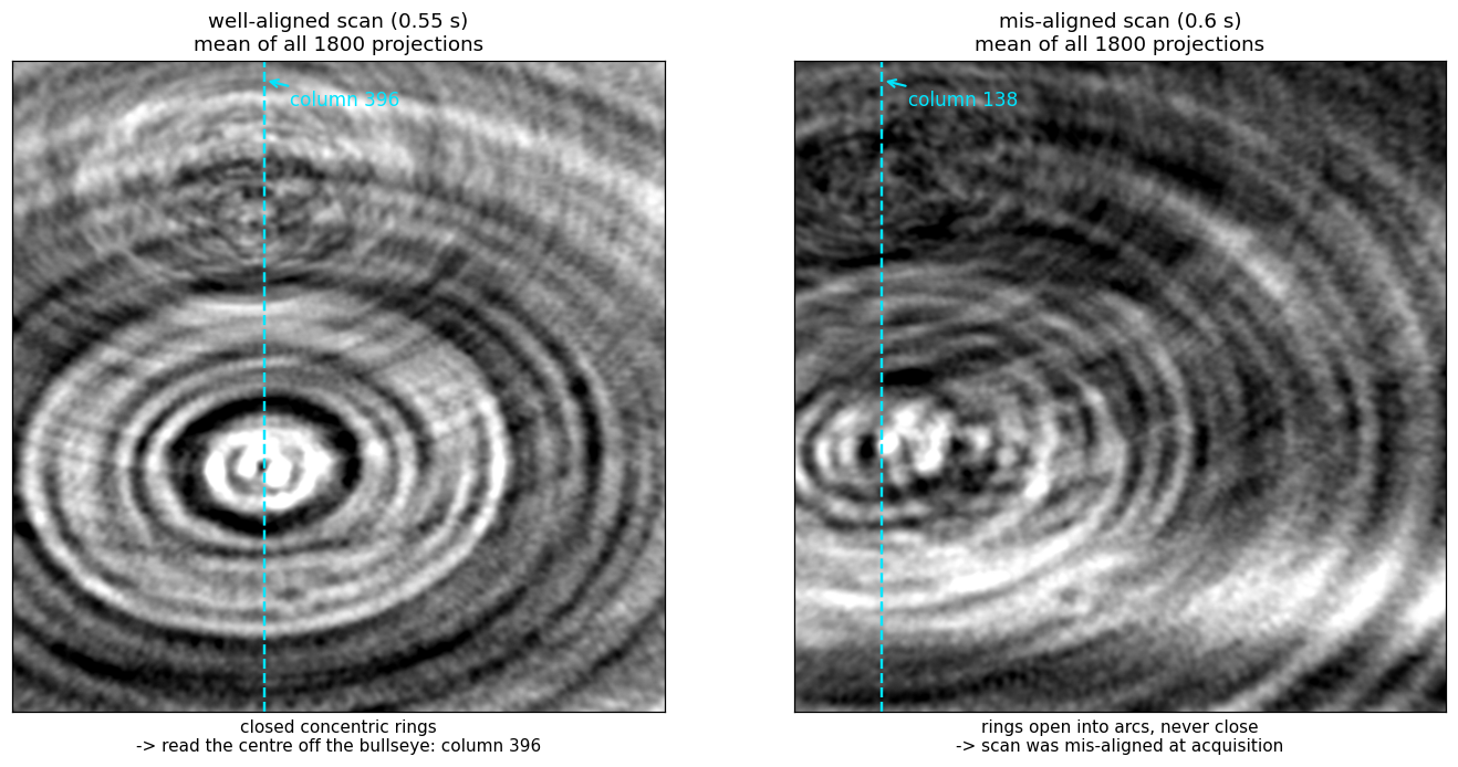
object point at radius r from the axis traces x(θ) = c + r·cos(θ + φ) across
the detector, so averaging over a full turn smears each point into a ring
centred on the rotation axis. The mean projection is a bullseye, and its
centre column is c.
def mean_proj(path, step=10):
    with h5py.File(path, "r") as f:
        w = f["exchange/data_white"][:].astype(np.float32).mean(0)
        d = f["exchange/data"]
        acc, n = None, 0
        for i in range(0, d.shape[0], step):           # every 10th frame is plenty
            m = -np.log(np.clip(d[i].astype(np.float32) / w, 1e-4, None))
            acc = m if acc is None else acc + m
            n += 1
    return acc / n
Read the bullseye column by eye. That is the whole method, and on the well-aligned scan the eye lands within a few pixels of the answer that a full reconstruction sweep produces.
The rings are also the alignment check
- Closed, concentric rings → the scan is aligned; the bullseye column is the center.
- Rings that open into arcs and never close → the sample was not aligned to
the rotation axis at acquisition. No choice of
--center/--lamino_anglerecovers this; it is a property of the measurement.
Automating it (and why the eye still goes first)
Concentric rings are mirror-symmetric about the axis column, so registering the
mean projection against its own left–right flip, a mirror about column
(nx − 1)/2, gives dx = 2c − (nx − 1):
def ring_center_col(M):
    A = M - M.mean()
    B = A[:, ::-1]
    cc = np.fft.fftshift(np.fft.irfft2(np.fft.rfft2(A) * np.conj(np.fft.rfft2(B)),
                                       s=A.shape))
    ny, nx = A.shape
    prof = cc[ny // 2 - 2 : ny // 2 + 3].sum(0)        # rings -> peak on the mid row
    i = int(np.argmax(prof))
    y0, y1, y2 = prof[i - 1], prof[i], prof[i + 1]     # parabolic sub-pixel
    d = (y0 - y2) / (2 * (y0 - 2 * y1 + y2))
    return (nx - 1 + (i + d) - nx // 2) / 2
Measured: 397.0 vs a known 396 (+1.0 px) on the aligned scan. On the mis-aligned scan it returned 281 vs a true 138 — the incomplete arcs on one side dominate the global correlation and drag the peak, while a human still reads the bullseye at 138 without difficulty.
So: eye first, correlation second, and treat a disagreement between them as the misalignment flag rather than as a number to average.
2. Coarse sweep with reconstructions
Take the column from §1 as the starting point and sweep. Two properties of the scoring are load-bearing; both were learned by getting them wrong first.
-
Reconstruct from the FULL projection set. On a 1/3 subsample the streak noise dominates and the focus metric tracks streaks instead of the sample.
-
Prep exactly once.
normalize_datasetalready ends in the minus-log; a secondminus_logon its output amplifies the noise floor everywhere the line integral is near zero while leaving the sample recognisable. On the aligned pouch scan the double-prepped volume ranked a pure-noise plane 1.7× above the eye-confirmed electrode, which made the whole-volume max unusable and was misread as a defect of the focus metric itself; with the prep fixed, the same metric puts the sample ≈6× above the noise floor and the unbanded tilt scan resolves 44° on its own (3.0× span over 36..52°). -
Score inside the sample's z band, carried to each tilt through the detector rows (
tomoxide align --focus_z LO:HI). Optional but load-bearing twice over: it is what the reference workflow does, and it keeps the score on the sample wherever structured noise still competes. A band cannot be fixed in z, though — the in-focus layer moves with the sample height and with the tilt: the sample's focus spike sits at z 837 / 890 / 956 at tilts 40° / 44° / 48° (volume depths 1338 / 1424 / 1532).The resolution is that the sample's detector rows do not move — they are a property of the data, not of the reconstruction. On the axis the back-projection samples row
v − nz/2 = cos(tilt)·(z − rh/2), so state the band once, at the tilt of the reconstruction you read it from, and map it into each candidate's own volume (tomoxide align --focus_z LO:HI;recon::center::SampleBandin the library). The mapping lands on the measured spikes to ~1 px: carrying the 44° band predicts 836 / — / 957.
Focus score per slice: mean |∇|² inside a 0.92-FOV disk; take the mean over
the band. Correct geometry sharpens every slice the sample is on; wrong
geometry blurs them all. The best single slice is not the score: each slice
peaks at its own candidate by what it holds (on a phantom rolled 2°, single
slices peak from 1.1° to 2.6° and the best one at 2.4°; their mean, at 2.0°).
The centre sweep takes the same mean (PreppedStack::center_sweep): on a
quartz scan eleven slices of one band peaked from 1045 to 1063 px and the
band's mean at 1055.9, where the three sharpest slices agree to 1.2 px. Read the band off one
reconstruction at your prior geometry — §3's eye check says which slices carry
round particles — or off the focus-by-slice profile the tilt scan reports.
The symptom of a broken search is a monotone surface with the argmax pinned to a grid corner. That means the metric has no focus signal to lock onto — widen the range or fix the scoring; do not report the corner as an optimum. A real optimum looks unimodal:
center  125    130    135    140    150      (tilt 45)
focus  5.18   5.55   5.89   5.92   5.65      (×1e-7)
3. Confirm visually, without the metric
Render the candidate centers side by side, each windowed to its own
p0.5/p99.5 percentiles, with a zoom. A window taken from one volume and applied
to another saturates the higher-contrast one into a fake-crisp binary look.
At the correct center the particles are round; a few tens of pixels away they smear into elongated dashes arranged in a swirl. This is unambiguous by eye and it is the check that catches a metric which has locked onto truncation artefacts rather than focus. In the worked example below, eye and metric agreed — which is the point of running both.
4. Fine 2D refine
Only now refine (center, tilt) together on a small grid. Small is the whole
point: both responses are broad, so a wide grid does not find an answer faster, it
finds a wrong one.
- Tilt: on the example data, 44/45/46 spanned 5.84/5.92/5.76 (×1e-7) — a ±1° error costs ~2%.
- Center: no sharper. Do not read the ~40%-per-50px figure that used to sit here — it was never measured. What was: on the aligned pouch scan (known axis 396, tilt 44°), a 21 px error cost 0.34%, and widening the sweep to ±40 px grew the curve three lobes whose highest stood at 417 — the wrong one, by a margin no rail check can see. Narrowed to ±8 px around the axis from §1, the same code returns 395.75.
So a (center, tilt) sweep refines a prior; it does not find one. Get the
center from §1's rings first, tilt second, and keep both grids tight enough that
there is only one lobe in them. recon::center::judge_sweep enforces this — it
returns no value from a curve with a rival lobe, and none from one that only rises.
5. Sanity check: the angular range
If the geometry search will not converge, verify the sweep is what the filename
claims. Rewrite exchange/theta to linspace(0, R, nproj, endpoint=False) for a
few R, reconstruct, and score:
R (deg)   350      355      360      365      370
focus    1.36     1.60     1.97     1.57     1.38     (×1e-6, aligned scan)
A correct range is a sharp peak — 360° beats ±10° by ~1.4× and beats 270°/450° by 5–8×. Run this at a center you have already established: the same scan scored at a wrong center gives a meaningless range curve.
6. Methods that failed validation — do not retry
Each of these was tried on the scan with the known center and did not reproduce it. They are recorded so the next person does not spend the time again.
| Method | Result on the known-center scan | Why it fails |
|---|---|---|
| 0°/180° mirror registration | scattered 395…607 across projection pairs (true: 396) | The tilted axis has a component along the beam, so a 180° rotation is not a mirror of the object. The symmetry the method assumes does not exist in laminography. |
| 1-D column-profile symmetry of the mean projection | 847 (true: 396) | The sample is wider than the FOV. Truncation destroys the symmetry of the 1-D profile; the 2-D ring pattern survives it. Use the rings, not the profile. |
| Sub-sampled (1/3) projections + fixed z band | monotone surface, argmax at a grid corner | Both failure modes of §2 at once. |
7. Worked example — the 2026-02-25/26 pouch pair
Two laminography scans of the same pouch cell, one day apart. They are separate
experiments, not variants: 18 hours and a remount apart, and the _re2 suffix
on the second marks it as a retake.
| 0.6 s scan (Feb 25) | 0.55 s scan _re2 (Feb 26) | |
|---|---|---|
| rings in the mean projection | open arcs, never close | closed, concentric |
| center (column) | 138 | 396 |
| tilt | 45° | 44° |
z_peak | 848 | 888 |
| focus (max over z) | 5.9e-07 | 2.0e-06 |
| slice contrast (p0.5–p99.5) | 0.028 | 0.046 |
The center moved by 263 px (in 2×-binned detector columns) between the two scans. Assuming the first scan's geometry transferred to the second is what made the initial searches fail; the ring picture would have shown it in one pass.
The Feb 25 scan reaches 30% of the Feb 26 focus and this is not recoverable by
reconstruction: it was mis-aligned at acquisition, which is what the open arcs
report and why the scan was retaken. Its raw projections are individually just as
sharp (mean |∇|² 0.003535 vs 0.003509, 0.7% apart, identical high-frequency PSD)
— sharp projections that are mutually inconsistent. In a single-turn scan time and
angle are the same variable, so acquisition misalignment cannot be separated from
angle-dependent structure by any choice of --center / --lamino_angle.
Not established. Both scans show
pearson(proj_0, proj_1799) ≈ 0.006 / 0.037where a 360° sweep should give ≈0.97; smoothing to σ=64 px lifts it to 0.77 / 0.74, so the coarse view does return (the 360° range is correct) while individual particles do not — they rearrange over the 64-minute acquisition. This appears in both scans, including the good one, so it does not explain the difference between them and no mechanism is claimed here.
tomoxide — Empirical Reconstruction Benchmarks
Companion to ALGORITHMS.md, which lists each method's design
properties. That guide notes a per-sample quality comparison had not been run;
this document is that comparison — measured reconstruction quality, speed, and
iteration behaviour of the analytic and iterative methods on real data.
Scope & honesty of the claims. Sections 2–7 (method quality) are from one real dataset (a low-contrast, smooth-object micro-CT scan) on one GPU (RTX 5000 Ada, CUDA, release build). They are a concrete data point, not a universal ranking — a high-contrast, piecewise-constant object (metal/pore samples) is exactly where total-variation shines more and the trade-offs shift. Regularisation strength
λ(--reg_par) is held at a common value except where a sweep is stated, so cross-method quality reflects behaviour, not each method's individually-tuned best. Reproduce on your own data before relying on a specific ordering.Sections 8–9 (backend/engine performance) are a separate axis — they compare the wgpu (Vulkan) and CUDA engines and the whole-volume vs streaming paths, not reconstruction quality. Their provenance differs (controlled/synthetic volumes, stated per section) and is called out inline. GPU clocks on this box are unlocked and swing widely, so those numbers are best-of-N (the highest clock wins); treat them as ratios, not absolute times.
1. Method & metric
- Data. A real micro-CT scan (
450projections over 180°, central 64-row band, 800 px wide). The native file is a beamline absorbance stack; it was converted to DXchange (data = exp(−absorbance), flat = 1, dark = 0,theta = linspace(0,180,nproj)), so tomoxide's minus-log recovers the measured absorbance. Three variants:- dense — all 450 views (well-conditioned);
- sparse — every 7th view = 65 views (ill-posed);
- noisy — sparse + simulated Poisson photon noise (
I₀ = 100, ≈ 10 %).
- Reference (quality proxy). Real data has no ground truth, so the yardstick is the dense 450-view SIRT@200 reconstruction of the same rows — the best available estimate of the true object. Sparse/noisy reconstructions are scored against it. This proxy is method-dependent — a dense FBP and a dense iterative recon of the same data disagree at Pearson r ≈ 0.73–0.81, so the reference silently favours recons that share its operator/prior. §10 removes that bias with a synthetic known-truth phantom.
- Metric. Pearson correlation (scale- and offset-invariant, so it is not fooled by the amplitude-convention differences between methods) is the primary discriminator; relative L2 is reported where informative.
- Semi-convergence caveat. Because the yardstick is the object (dense ref), quality-vs-iteration curves peak then decline: an iterative method first approaches the object, then converges onto the sparse data's own solution (streaks/noise absent from the dense ref) and moves away. This "distance to the true object" view is deliberate — it is what shows the practical optimal iteration count. Measured against the sparse method's own limit the curves would be monotone instead.
2. Analytic: FBP vs gridrec (CUDA)
Dense 450-view, 64 slices, 800².
| method | path | wall | quality (Pearson) |
|---|---|---|---|
fbp (parzen) | device-resident fused filter→backproject | 0.98 s | 0.870 |
fbp (ramp) | same | 0.94 s | 0.839 |
gridrec | cuFFT + host gridding (not device-resident) | 3.09 s | 0.731 |
- Kernels (nsys). FBP's GPU time is 88.5 %
backprojection_ker(the real O(N²·Nθ) work), with a small FFT-based filter pass. gridrec's GPU time is 82 % cuFFT (regular_fft/vector_fft) — no back-projection kernel, because the polar→Cartesian gridding runs on the host. gridrec's GPU kernel time is only ~11 ms (vs FBP 49 ms) yet its wall is 3.2× longer → it is host-bound, not a true GPU reconstruction. - Filter. FBP honours
--filter(apodisation); gridrec applies a pure ramp only (filter_nameis ignored — seerecon/gridrec.rs). - Amplitude. gridrec output ≈
0.0011 ×FBP — a different normalisation convention (gridrec is excluded from the CUDA convention unification). Orientation matches FBP (no flip). - Verdict. On CUDA, FBP wins on this box: faster (fused GPU back-projection) and higher fidelity (apodisation). gridrec's O(N² log N) advantage is unrealised while its gridding is host-side.
3. FBP apodisation filter
Relative high-frequency energy (clean, ramp = 1.0):
ramp 1.00 > shepp 0.56 > cosine 0.12 > hamming 0.057 > cosine2 = hann 0.039 > parzen 0.003.
(none = no filter = 1/r blur, not a valid reconstruction.)
| filter | clean Pearson | noisy Pearson |
|---|---|---|
| ramp | 0.839 | 0.068 |
| shepp | 0.883 | 0.078 |
| cosine | 0.917 | 0.105 |
| hamming | 0.920 | 0.125 |
| cosine2 / hann | 0.908 | 0.131 |
| parzen | 0.870 | 0.262 |
- Sharpness ↔ noise trade-off. On clean data quality is U-shaped —
mid apodisation (
hamming/cosine) is best;rampis too noisy,parzenover-smooths real detail. On noisy data the order flips: strong apodisation (parzen) wins,rampis worst. - The default
parzenis a safe choice for noisy real data but slightly over-smooths clean, well-sampled data (0.870 vs hamming 0.920). hannandcosine2are numerically identical in this implementation (Hann window = cos²).noneis not a reconstruction: it looks high on the noisy metric (0.648) only because a smooth blur happens to correlate with a smooth reference — no real detail is recovered.
4. Iterative methods at equal iterations (40 iters, 65-view sparse)
4.1 Speed & feasibility
- Device-resident methods (
sirt,cgls,mlem,osem,tv,grad,tikh,pml_*,ospml_*) are all comparable, ~2.6–5.9 s at 40 iters (cglsandsirtare near-identical per iteration — each is one forward + one back-projection;cgls40 iters 5.44 s vssirt5.87 s). art/bartare host row-action code (not device-resident): a single 800² slice at 40 iters did not finish in 115 s (full volume > 2 h). Impractical at this resolution — reserve for small images.
4.2 Data-model applicability — negative projections
The real low-contrast sinogram is 29.5 % negative (weakly-absorbing sample → baseline near zero, noise dips below it). The emission/statistical family requires non-negative projections and blows up on it:
| family | on raw (has negatives) |
|---|---|
sirt, cgls, tv, grad, tikh (algebraic / least-squares) | robust (bounded) |
mlem, osem (multiplicative Poisson) | diverge (output ±thousands, relL2 44–50) |
pml_*, ospml_* (penalised-ML) | NaN |
This is a data-model mismatch, not a bug: MLEM's b/(Ax) update goes wrong
when b < 0. Clamping to non-negative makes MLEM reconstruct fine (0.787).
4.3 Handling the negatives
Negative attenuation is physically impossible, so floor projections at 0 (clip transmission ≤ 1). Then all methods are stable:
| method | clean | noisy | family |
|---|---|---|---|
| sirt | 0.836 | 0.535 | algebraic |
| tv (λ=0.001) | 0.818 | 0.628 | total-variation |
| pml_hybrid / ospml_hybrid | 0.788 | 0.320 | penalised-ML |
| mlem / osem | 0.787 | 0.319 | Poisson EM |
| cgls † | 0.770 | 0.266 | Krylov least-squares |
| grad / tikh | 0.670 | 0.647 | least-squares (BB) |
† CGLS is past its peak at 40 iters — as the fastest-converging method it reaches its best (clean 0.839 at 10 iters) far earlier and then semi-converges hard, so a 40-iter snapshot understates it on clean data and buries it on noisy. See §4.5 for its curve; do not read its row here as its ceiling.
- Clean: SIRT > TV > emission family > GRAD/TIKH (the last under-converged at 40 iters). Noisy: GRAD/TIKH ≈ TV > SIRT ≫ emission (multiplicative methods are noise-sensitive, and flooring 38 % of noisy rays to zero adds bias).
- Flooring is not free for the least-squares family — it discards ~30 % of rays, nudging SIRT clean 0.843 → 0.836. It enables the emission methods at a small cost to the algebraic ones.
- Do NOT clip to a small positive ε instead of 0. Mapping negatives to +ε
(leaving positives) destabilises the emission methods — clean MLEM 0.787 →
0.688, PML back to NaN, and ε-sensitivity is chaotic (MLEM: ε1e-4 → 0.787,
1e-3 → 0.688, 1e-2 → 0.802). Cause:
b/(Ax)blows up where the model predictsAx ≈ 0butb = ε > 0.sirt/tv/gradare identical under ε vs 0 (additive updates). Floor to exactly 0. mlem == osem == pml == ospmlpairwise on this data (Poisson family, default subsets);grad == tikh(Tikhonov's L2 term is negligible at λ=0.001, reducing it to plain BB gradient descent).
4.4 Does any method "catch up" to SIRT with more iterations?
Sweep on floored clean data, Pearson vs dense ref:
| iters | SIRT | MLEM | GRAD |
|---|---|---|---|
| 40 | 0.836 | 0.787 | 0.670 |
| 80 | 0.838 | 0.751 | 0.675 |
| 160 | 0.817 | 0.716 | 0.683 |
| 320 | 0.791 | 0.683 | 0.697 |
| 640 | 0.776 | 0.656 | 0.717 |
- MLEM never reaches SIRT. Its whole curve sits below SIRT's, and — like SIRT — it semi-converges, so more iterations widen the gap. Different objective (Poisson likelihood), lower/earlier plateau.
- GRAD/TIKH climb very slowly. At 640 iters (0.717) they are still below even
SIRT@640. They minimise the same
‖Ax−b‖²as SIRT, so they meet SIRT only at full least-squares convergence (thousands of iters) — by which point semi-convergence has pulled that shared quality below SIRT's early peak. - Takeaway: SIRT@~40–80 is near-optimal here and cannot be beaten by throwing iterations at MLEM or GRAD.
4.5 CGLS — fastest convergence, but no regularization
CGLS solves the same ‖Ax−b‖² normal equations as SIRT/GRAD, but as a Krylov
method (optimal step + conjugate directions) it converges in far fewer
iterations. That speed is a double-edged sword: with no regularizer it races to
the least-squares solution of the sparse/noisy data, so it peaks early then
semi-converges harder than SIRT.
Pearson vs the dense ref, per-slice mean, floored data:
Clean:
| iters | CGLS | SIRT |
|---|---|---|
| 5 | 0.833 | 0.742 |
| 10 | 0.839 (CGLS peak) | 0.777 |
| 20 | 0.790 | 0.812 |
| 40 | 0.770 | 0.836 (SIRT peak) |
Noisy:
| iters | CGLS | SIRT |
|---|---|---|
| 5 | 0.433 (CGLS peak) | 0.705 |
| 10 | 0.285 | 0.696 |
| 20 | 0.267 | 0.643 |
| 40 | 0.266 | 0.535 |
- On clean data CGLS is the convergence-speed winner. Its peak (0.839 @10)
matches SIRT's eventual best (0.836 @40) in 4× fewer iterations — and since
a CGLS iteration costs the same as a SIRT one, that is a real wall-time win:
cgls --num_iter 10= 2.01 s for 0.839 vssirt --num_iter 40= 5.87 s for 0.836 (≈2.9× faster at equal-or-better quality). This is the payoff over FBP-seed warm-start (§6), which saved iterations but not wall-time on this GPU. - Early stopping is mandatory. CGLS has no prior to resist semi-convergence, so past its peak it falls off faster than SIRT (clean 0.839→0.770 by 40).
- On noisy data CGLS is the worst of the algebraic family. It peaks at just 5 iters (0.433 — already below SIRT@5's 0.705) and collapses to 0.266, because it fits the photon noise almost immediately. For noisy/low-dose data use TV (§5), whose prior is exactly what CGLS lacks.
- Use CGLS for well-posed / densely-sampled data where you want the least-squares answer fast, with a small iteration count and early stopping.
5. SIRT vs TV by iteration count
The two best methods on this data behave fundamentally differently with iterations.
Clean (floored, λ=0.001):
| iters | SIRT | TV |
|---|---|---|
| 40 | 0.836 | 0.818 |
| 80 | 0.838 (SIRT peak) | 0.842 |
| 160 | 0.817 | 0.850 (TV peak) |
| 320 | 0.791 | 0.843 |
| 640 | 0.776 | 0.827 |
Noisy (floored):
| iters | SIRT | TV (λ=0.001) | TV (λ=0.1) |
|---|---|---|---|
| 40 | 0.535 | 0.628 | 0.772 |
| 80 | 0.415 | 0.502 | 0.762 |
| 160 | 0.329 | 0.387 | 0.733 |
| 320 | 0.283 | 0.317 | 0.702 |
| 640 | 0.266 | 0.285 | 0.679 |
- SIRT converges fast but has a delicate optimal stopping time. It peaks early (~40–80 iters) then declines via semi-convergence — gently on clean (−0.062 by 640), catastrophically on noisy (0.535 → 0.266, −0.269). Early stopping is mandatory.
- TV reaches a higher, later, flatter plateau — its total-variation prior resists semi-convergence. Clean: peak 0.850 @160 (drop only −0.024). Crossover: SIRT wins ≤ ~60 iters (faster early), TV wins ≥ 80.
- But TV's robustness depends on λ. At too-low λ (0.001) TV crashes on noise like SIRT; at an adequate λ (0.1) it stays high (0.772 → 0.679). TV converts the brittle stopping-time problem into a more forgiving λ-tuning problem — once λ fits the noise level, iteration count is forgiving.
6. Warm-start chaining (--algorithm a,b,…)
- FBP→SIRT warm-start benefit is view-count / conditioning dependent: ~0.7 % at 450 views (well-sampled), ~5 % and roughly halved iterations at 65 views (ill-posed). On this fast GPU at 800² it is not a wall-time win — the extra FBP stage costs more than the iterations it saves.
- More stages is not automatically better. A 3-stage
fbp,sirt,tvdoes not reliably beat 2-stage on this data: clean →fbp,sirt; noisy →fbp,tvortv(inserting a SIRT stage between FBP and TV hurts under noise — SIRT fits noise the later TV must undo). FBP-seeding helps SIRT but not TV (TV's prior dominates its initial guess). - Per-stage iterations:
--algorithm fbp,sirt:30,tv:10gives each iterative stage its own budget (seeALGORITHMS.mdand the README).
7. Practical selection guide
- Analytic, quick look:
fbp(device-resident, fast). Pick the filter for the data —hamming/cosinefor clean/well-sampled,parzen(default) for noisy. Preferfbpovergridrecon CUDA (faster, higher fidelity, correct scale). - Iterative, attenuation data that can go negative:
sirt(fast, accurate, robust; stop at ~40–80 iters) ortv(higher ceiling and far more iteration-robust onceλfits the noise). Avoidmlem/osem/pml/ospmlunless projections are guaranteed ≥ 0 (emission tomography, or floor to 0 first). Neverart/bartat high resolution. - Well-posed / dense data, want the least-squares answer fastest:
cglswith a small iteration count and early stopping (peak ~10 iters here, ≈2.9× less wall-time than SIRT for equal quality). No regularizer, so not for noisy or very sparse data — there it fits noise almost immediately (§4.5); usetvinstead. - Noisy / low-dose:
tvwith an adequately strongλ(do a short λ sweep); it resists the semi-convergence that collapses SIRT (and, worse,cgls). - Warm-start: worth it for sparse/limited-angle data (
fbp,sirt); match the chain to the data (fbp,tvfor noise), and remember iteration savings ≠ wall-time savings on a fast GPU.
8. Backend performance — wgpu (Vulkan) vs CUDA
tomoxide's recon runs on three engines (CPU, CUDA, wgpu). wgpu is the portable
GPU path (Vulkan/Metal/DX12); on this NVIDIA box it runs through Vulkan. The two
GPU engines are numerically equivalent — Pearson(cpu, wgpu) = 1.0 on every
ported method — so this section is purely about speed, not fidelity.
Per-slice kernel gap, controlled 1024² volume, nz = 2, RTX 5000 Ada,
best-of-N (ratio = wgpu wall ÷ CUDA wall; < 1 means wgpu is faster):
| algorithm | wgpu ÷ CUDA | why |
|---|---|---|
fbp / linerec | ~1.1× (parity) | back-projection reads are already coalesced; the FBP filter is device-resident (pack/pad/crop on-GPU) |
fourierrec | ~1.6× | was ~2.6–2.8× when the Fourier gather-scatter emulated atomicAdd via a CAS loop; native f32 atomics (below) removed that penalty — the residual is per-dispatch submission overhead (~19 submits/chunk) |
lprec | ~0.8× (wgpu faster) | both engines are dominated by the shared host build_grids precompute, not GPU throughput |
gridrec | ~1.5× | both host-bound (polar→Cartesian gridding runs on the host on both engines); neither is a true device reconstruction |
sirt | ~0.5× (wgpu faster, est.) | the forward projector — a per-voxel atomic scatter, ~95 % of SIRT's wall — sped up 6.4× with native f32 atomics; measured wgpu SIRT(10) 235 ms vs the recorded CUDA ~515 ms (CUDA not re-measurable on this build) |
- Native f32 atomics (wgpu ≥ 24,
SHADER_FLOAT32_ATOMIC). The old structural gap — WGSL had no float atomic, so every scatter accumulation (forward projection, fourierrec gather/wrap, lprec gather) paid a compare-exchange emulation loop with 2–3× the memory traffic of CUDA's one nativeatomicAdd— is gone on hardware exposing VulkanVK_EXT_shader_atomic_float. Same-build A/B (CAS forced viaTOMOXIDE_WGPU_NO_F32_ATOMICS=1vs native, release, 1024² nz = 2): forward project 139.5 → 21.0 ms (6.6×), SIRT(10) 1515 → 235 ms (6.4×), fourierrec 32.5 → 23.0 ms (1.4×). Devices without the feature (Metal, older drivers) transparently fall back to the CAS variant. - fbp/linerec are at CUDA parity — the fused device-resident analytic path (filter → back-projection kept resident) closed the old 1.7× marshaling gap.
- lprec and gridrec are host-precompute / host-gridding bound, so the engine choice barely matters — the lever there is the shared host code, not the GPU.
9. wgpu device-resident streaming (whole-volume vs streaming)
The wgpu whole-volume reconstruct() wall is 60–82 % host cost: the
projection-domain minus-log runs through a wgpu round-trip (the whole projection
volume is uploaded just to run one elementwise kernel, then downloaded) plus a
full-volume projection→sinogram host transpose — neither is GPU-recon work. The
streaming path removes both: it normalises each chunk on the CPU (parallel,
memory-bound minus-log — no GPU round-trip), transposes just that chunk, runs the
fused device recon (one PCIe hop up, one down), and overlaps disk read/compute/write
across chunks.
A/B on a synthetic 600 × 128 × 512 DXchange stack, TIFF output, chunk = 8,
RTX 5000 Ada via Vulkan, best-of-3:
| method | whole-volume | streaming | speedup |
|---|---|---|---|
fbp | 1.71 s | 1.20 s | 1.43× |
fourierrec | 2.52 s | 2.35 s | 1.07× |
lprec | 2.18 s | 1.24 s | 1.76× |
- The win scales with the host round-trip the whole-volume path pays.
lprecgains most (1.76×) because its whole-volume path paid the minus-log round-trip over the entire projection volume;fourierrecgains least (1.07×) because its per-chunk wall is dominated by the GPU gather (§8), so removing host cost moves a smaller fraction. - Parity: streaming output == whole-volume output, per-slice
Pearson > 0.999, including the partial trailing chunk (verified intests/wgpu_streaming.rsfor fbp / fourierrec / lprec). - Streaming also enables reconstructions that whole-volume cannot — a large
fourierrecvolume whose oversampled2n × 2ngrid would exceed the wgpu max-buffer limit fits chunk-by-chunk. - Streaming does NOT close the per-slice kernel gap in §8 — that gap is
kernel-throughput-bound and measured with data already resident. A follow-up
device-transpose lever was measured and dropped:
fbpstreaming is I/O-bound (compute ≪ wall, the transpose is already hidden behind the read/write threads) andfourierrecis recon-bound (transpose < 10 % of a recon-dominated chunk), so moving the transpose on-device buys nothing on this box.
lprecstreaming needs the DXchange/exchange/thetastored in degrees (the reader convertsdeg/180·π, matching tomocupy); a file with radian-stored angles fails lprec's equal-spacing guard. This is a fixture convention, not a code limit.
10. FBP vs iterative: accuracy against a known-truth phantom
FBP often looks sharper and more detailed than an early-stopped iterative recon, yet on real data (§4–5) the two score "similar". This section settles two questions the real-data yardstick cannot: is FBP's apparent extra detail accuracy or just contrast, and is a well-run iterative method genuinely closer to the true object? It is the only section here scored against a known ground truth.
Scope of the claims. One Shepp–Logan-based phantom family (a piecewise-constant variant and a smooth textured variant), 2D central slice, parallel-beam,
parzenFBP. The phantom is synthetic — real specimens differ in structure and noise. The real-data disagreement figures (§10.1) are from a single NCA XANES scan. Treat the directions as robust and the exact numbers as one-sample.
10.1 Why real data cannot answer this
The §1 quality proxy is a dense iterative recon — but "dense truth" is itself method-dependent. On a real 1800-view NCA scan, dense reconstructions by different methods disagree (mutual Pearson r of the same rows):
| dense ref (1800-view) | FBP | CGLS-20 | SIRT-150 | TV λ.02 |
|---|---|---|---|---|
| FBP | 1.000 | 0.727 | 0.804 | 0.808 |
| CGLS-20 | 0.727 | 1.000 | 0.951 | 0.919 |
| SIRT-150 | 0.804 | 0.951 | 1.000 | 0.993 |
| TV λ.02 | 0.808 | 0.919 | 0.993 | 1.000 |
FBP sits ~0.8 from every iterative recon; the iterative methods agree with each other at 0.92–0.99. There is no method-neutral truth in real data: whichever dense method you crown as reference biases the score toward recons that share its operator/prior. A synthetic phantom is the only way out.
10.2 Phantom protocol (inverse-crime-mitigated)
- Truth built at 2× (1600²): Shepp–Logan + resolution-bar groups. A second textured variant multiplies in a smooth sinusoid + radial-gradient modulation so the object is not piecewise-constant — this denies TV its home-field advantage.
- Generation grid ≠ recon grid: forward-project the truth, bin the detector 2× → 800, reconstruct at 800; score against the phantom binned to 800. The grid mismatch avoids the inverse crime (recon operator ≠ inverse of the exact generator).
- Noise: transmission-domain Poisson,
counts ~ Poisson(I₀·e^−sino). The sinogram is first normalised to peak attenuation ≈ 2.5 — without this the raw path integral (~500) makese^−sinounderflow and the noise becomesI₀-independent (a real bug we hit; watch for saturated sinograms). - Metrics vs known truth: affine-fit NRMSE (scale/offset-invariant, ↓) and mid-band structural correlation r_mid (band-limited complex correlation, ↑) — the accuracy analogue of FRC, but measured against truth rather than a second half.
Reproducibility ≠ accuracy. FRC / half-split correlation measures whether two halves agree, not whether they are right; a strong prior inflates FRC by biasing both halves the same way. Only a known truth separates the two — which is exactly why this section exists and §1–§9 (real data) cannot replace it.
10.3 Results — textured phantom, TV λ retuned per scale
NRMSE ↓ / r_mid ↑; best NRMSE per row in bold. TV's λ is the sweep winner at this sinogram scale (see finding 4).
450 views (well-sampled):
| noise | FBP | CGLS-30 | SIRT-150 | TV (best λ) |
|---|---|---|---|---|
| noiseless | 0.275 / 0.828 | 0.148 / 0.945 | 0.258 / 0.880 | 0.127 / 0.955 (λ 3e-4) |
| I₀=8000 | 0.278 / 0.808 | 0.284 / 0.867 | 0.263 / 0.853 | 0.154 / 0.918 (λ 1e-3) |
| I₀=3000 | 0.284 / 0.777 | 0.423 / 0.760 | 0.272 / 0.814 | 0.185 / 0.881 (λ 1e-3) |
120 views (sparse):
| noise | FBP | CGLS-30 | SIRT-150 | TV (best λ) |
|---|---|---|---|---|
| noiseless | 0.291 / 0.766 | 0.273 / 0.782 | 0.288 / 0.799 | 0.203 / 0.800 (λ 1e-3) |
| I₀=8000 | 0.302 / 0.711 | 0.315 / 0.714 | 0.300 / 0.739 | 0.220 / 0.764 (λ 1e-3) |
| I₀=3000 | 0.320 / 0.640 | 0.370 / 0.630 | 0.318 / 0.663 | 0.232 / 0.707 (λ 3e-3) |
FBP, CGLS and SIRT are linear, so scaling the sinogram leaves their scores unchanged; TV is nonlinear and its λ must be retuned for the scale (finding 4).
10.4 Findings
- A properly-regularised iterative method (TV, λ tuned to the noise) is closest to the truth in every regime — sparse or dense, clean or noisy — including on the textured phantom built to deny TV its piecewise-constant advantage. At 450 views it roughly halves FBP's NRMSE (0.13–0.19 vs ~0.28).
- "Iterative" is not one thing — configuration decides. Unregularised, fixed-iteration CGLS is the best method at high SNR (450 noiseless: 0.148) but the worst under noise (450 I₀=3000: 0.423 > FBP 0.284) — it fits noise almost immediately (matches §4.5). SIRT-150 tracks FBP: robust, never disastrous, never best.
- FBP is the noise-robust floor. Its NRMSE barely moves across the whole
noise range (450: 0.275 → 0.284) because the ramp +
parzenapodisation caps what it passes — but it is never the most accurate. Its extra apparent detail is high-frequency contrast (real edges + streaks + noise), which reads as "sharper" while lowering fidelity. Sharpness ≠ accuracy. - TV's λ is data-scale-dependent. It must be retuned when the sinogram amplitude changes, and increased as noise rises (here 3e-4 → 1e-3 → 3e-3). A λ fitted at one amplitude over-regularises by orders of magnitude at another — the same trap as scoring a scaled recon without re-fitting λ.
This corroborates §7's selection guide from the truth side: tv with a fitted λ
for noisy/sparse data; cgls only for well-posed/dense data at a small iteration
count; sirt as the robust default; fbp for a fast, safe look — accepting it
will not be the most accurate, and its sharper appearance is contrast, not
recovered structure.
Sections 2–7 were reproduced with the
cudafeature build on real data; §10 on real data (§10.1) plus synthetic known-truth phantoms, same build; sections 8–9 with thecudaandgpu-wgpubuilds on the controlled/synthetic volumes stated inline. Scripts and intermediate reconstructions are not committed. Re-run on your own sample and GPU before committing to a method or an engine — see the scope note at the top.
tomoxide — GUI design (tomoxide-gui)
This document is the design for a desktop GUI for tomoxide: a new crate
crates/tomoxide-gui built on rsplot (egui 0.34 + wgpu scientific plotting,
a silx port) for every scientific view, and on rsplot's sibling crate rsdm
(a PyDM-style EPICS display/data-engine layer) for live PVAccess data. It
covers three workflows in one application:
- Offline — open a DXchange HDF5, tune parameters on a single-slice preview, find the rotation axis, reconstruct the full volume, browse the result.
- Live streaming — subscribe to a tomoScanStream-style PVA projection stream and reconstruct ortho-slices continuously while the operator nudges the rotation center (the tomostream operating model).
- Spectroscopic (XANES) — take a stack of reconstructed volumes acquired across an absorption edge, fit each voxel's spectrum, and map the chemical state (edge-shift / white-line energy) in 3-D.
Intellectual-property note. The workflow of the commercial Octopus Reconstruction package (single-slice tune loop, candidate-montage parameter evaluation, pre-flight resource checks, stack rescaling) and the operator model of APS tomostream (live ortho-slices, live center tweak, click-to-set) are used as concept references only. No text, artwork, screenshots, or screen layouts are copied; every screen here is an original composition of rsplot widgets around tomoxide's actual API surface.
1. Application shell
An eframe application (wgpu renderer — required by rsplot) with:
- a left mode rail (
egui::SidePanel) selecting one of seven modes: Data · Tune · Center · Run · Output · Live · XANES; - a persistent bottom log pane (collapsible): every job with its parameters, timing, and outcome — the session history;
- a status bar: resolved backend (
Engine::name()), GPU inventory (cuda::selected_devices()/cuda::device_name()), last recon time.
No docking framework in v1 — plain egui panels; rsplot's detached windows
cover "pop this view out". All modes share one Project (the parameter
model, §5) and one recon worker (§4).
2. Screens
2.1 Data — dataset browsing
- Open a DXchange HDF5 via a native file dialog; the worker calls
open_dxchange(path),read_sizes(),read_theta(). - Metadata card: nproj / nz / nx / nflat / ndark, theta start/end/step, raw size estimate.
- Projection browser: rsplot
StackViewover the projections. ItsFrameLoadertrait isSend + Syncbut rust-hdf5'sH5Fileis!Send, so the loader is a channel client:load(i)sends a request to the worker thread (which owns the reader) and blocks on the reply. StackView's lazy loading keeps this cheap. Flat/dark frames are viewable through the same view via a source selector. - Theta plot:
Plot1Dof the angle array (irregular or missing angle sets are visible at a glance). - Sinogram inspector: pick a detector row →
ImageViewof the[nproj × nx]sinogram (side histograms/colorbar off; anImageView, not a barePlot2D, so the crosshair readout can show the pixel value under the cursor viavalue_changed— the silxPositionInfo"Data" column).
2.2 Tune — the single-slice preview loop
The core interaction (the Octopus tune-loop concept mapped onto tomoxide):
- Left: a decimated projection thumbnail (
Plot2D) with a draggable horizontal line selecting the preview slicez. - Middle: the parameter panel — tabbed groups mirroring the CLI's
conceptual grouping, with the Octopus conventions of greying out
irrelevant fields and "auto" checkboxes mapping to
None:- Geometry — rotation axis (auto checkbox →
None= midline),lamino_angle; - Algorithm — algorithm combo including the chain syntax
(
fbp,sirt:30,tv:10) via a small chain builder; filter combo (ramp/shepp/cosine/cosine2/hamming/hann/parzen);num_iter/reg_pargreyed out for analytic algorithms; - Prep — stripe method + only the selected method's parameters enabled
(
fw_*,ti_*,sf_*,vo_*); phase-retrieval method + physics (pixel_size,propagation_distance,energy,alpha,db,w); - System — backend (Auto/Cpu/Cuda/Wgpu), dtype (f32/f16), chunk size with the tuned-cache value shown, per-slice timing of the last preview and the extrapolated full-volume estimate.
- Geometry — rotation axis (auto checkbox →
- Right (dominant): the current single-slice preview as an rsplot
ImageView— its crosshair reads out the pixel value under the cursor (value_changed, the silxPositionInfo"Data" column) and its interactive colorbar (value histogram + draggablevmin/vmax) sets the display range. A "Pin" button (or holding Space) snapshots the current result together with its parameters and switches the pane to rsplotCompareImages— the current preview as image B against the pinned one as image A; split/subtract/A-B modes give instant parameter comparison, with rectangle-ROI stats and line profiles. - Auto-recon toggle: debounced (~300 ms) re-reconstruction on any parameter change — viable because one analytic slice on the GPU is sub-second.
- λ sweep (L-curve regularization tuner): shown only for algorithms whose
reg_par[0]is a regularization strength λ (tv,grad,tikh,pml_*,ospml_*). Reconstructs the current slice once per λ across a log-spaced grid (all other parameters fixed), then plots the L-curve — data residual‖A x − b‖₂(the exact fidelity term the solver minimizes) against the reconstruction's isotropic TV seminorm (roughness), both in log₁₀. A floating window shows the per-λ montage (ImageStack) over the L-curve (Plot1D); the corner is highlighted as the suggested λ and a click snaps to any point, "Use selected λ" writes it back toreg_par[0]. The guidance is deliberately the L-curve corner, not a sharpness auto-pick: λ is not solvable like the rotation axis, sharpness decreases monotonically with λ, and on real data there is no ground truth — so the pick stays the user's (the accuracy rationale isBENCHMARKS.md§10).
Execution path: the worker preps row z with tomoxide::prep_band(z, z + 1)
and reconstructs that one sinogram with recon::recon, for every algorithm
including the iterative ones. Phase retrieval couples rows, so prep_band
reads prep::phase::margin_rows more on each side and drops them before
stripe removal: the center row's retrieval is exact and the preview stays
one-slice cheap however wide the kernel is.
2.3 Center — finding and evaluating the rotation axis
Three complementary tools on one screen:
- Auto buttons — Vo (
find_center_vo, the workhorse), Entropy (find_center), Phase-correlation (find_center_pc), and SIFT (find_center_sift, shown only when thesift-centerfeature is compiled in). Each runs on the worker against the current preview slice and proposes a value with an explicit "accept" step. - Sweep montage — the Octopus parameter-evaluator concept, backed by
the existing
recon::center::write_center(tomo, theta, backend, cen_range, ind, mask, ratio) -> (Vec<f32>, Array3<f32>): the user sets center ± range ± step; the candidate reconstructions become aStackView(frame label = candidate center) next to aPlot1Dof a per-frame sharpness metric (image standard deviation) with click-to-pick. A "refine" button re-runs the sweep centered on the pick with step/4. - Fine tweak — ±0.5 / ±0.25 px nudge buttons that immediately re-run the single-slice preview. The same control reappears in Live mode (tomostream's CenterTweak), where it applies on every loop.
2.4 Run — full-volume reconstruction
- Output: path, format (tiff/h5/zarr), dtype.
- Pre-flight panel (the Octopus System-tab concept): disk estimate
(
nz·ny·nx·dtypevs. free space), chunk from the CLI's tune cache (keyed by file/algorithm/dtype/GPU), wall-time extrapolated from the last preview — each with a green/red feasibility indicator. GPU picker (checkbox per device). - Execution is always a subprocess. The GUI spawns
tomoxide(the CLI) — one process per selected GPU with--start_row/--end_rowz-shards, exactly the CLI's own multi-GPU fan-out; one process for CPU or a single GPU too. Rationale: a single code path, the per-process cuFFT-plan/VRAM isolation is already the library's deliberate design, cancellation is process kill (no library hook needed on this path), and a CUDA OOM cannot take down the GUI. Requires the CLI addition--progress-json(§6 #4); the GUI tails one JSON line per completed chunk from each child. - Live progress: per-shard and aggregate progress bars, plus a
latest-slice view (
Plot2Dwithtry_update_image, zoom preserved) when the output is tiff (per-slice files are cheap to load as they appear). For h5/zarr output only the progress bars are shown — single-container writers are not shardable and the container is not valid until finalize; this limitation is accepted and documented. - Cancel kills the children; partial tiff output stays on disk and is noted in the log.
- Batch queue (phase 2): an ordered list of (dataset, recipe TOML) pairs run sequentially — each recipe being exactly the file the CLI consumes, so a queue tuned in the GUI is scriptable headlessly.
2.5 Output — result browsing
StackViewover the reconstructed volume with per-formatFrameLoaders implemented in the GUI (tiff directory via thetiffcrate; h5 through the worker-thread channel client; zarr chunk files directly).- 3D: rsplot
ScalarFieldView(isosurface) over a worker-built downsampled copy (≤ ~256³). - Rescale/export (the Octopus rescale concept): a volume histogram
(
Plot1Dwith a draggable min/max range) drives export of the stack to 8/16-bit tiff on a common gray scale. Pure GUI-side conversion.
2.6 Live — streaming ortho-slice reconstruction
The tomostream operating model, in-process:
- Connection panel: PVA channel addresses for projection / dark / flat /
theta (tomoScanStream conventions as defaults), connected through the
rsdmdata engine (its own tokio runtime). Frames land in a fixed-capacity ring buffer holding ~180° of projections plus theta and rolling dark/flat. - Recon loop on the worker: wakes on new frames or any parameter change,
assembles sinograms for the selected slice indices from the ring buffer,
reconstructs, and publishes to the UI (
try_update_image+request_repaint). - Views:
Plot2Dpanes with crosshair cursors marking the other slice positions, and click-to-set — clicking a position in one pane moves the other slice indices (tomostream's signature interaction, minus its NaN-line hack: rsplot draws real markers). - Parameters (re-read every loop, tomostream semantics): center + tweak up/down (live nudging), filter, ring removal (none/fw), slice indices, Paganin group, Start/Abort, recon-time and buffer-fill readouts.
- Honesty note: tomoxide today reconstructs Z slices cheaply
(analytic recon is per-slice independent), so live mode ships Z-only
first — one or several horizontal slices. The X/Y ortho panes require
new dedicated single-slice backprojection kernels (§6 #7; tomostream has
orthox/orthoyCUDA kernels, tomoxide does not). Incremental ring-buffer recon (obj += bp(new) − bp(old)) is an optimization (§6 #8); v1 recomputes the displayed slices each loop, which analytic GPU recon sustains at interactive rates for typical detector widths.
2.7 XANES — spectroscopic chemical mapping
The post-reconstruction spectroscopy workflow of the existing xanes_tools
pipeline, brought in-process. Input is a stack of reconstructed volumes, one
per photon energy across an absorption edge (Fe / Co / Ni K-edge, …); output
is a per-voxel chemical-state map — the fitted white-line / edge energy —
modulated by the edge jump (absorber thickness/density).
- Input. Either (a) the native product of the Run screen's batch
queue — one tomoxide output per energy (each a tiff directory /
.h5holding a single/exchange/data/.zarr) plus the energy list, or (b) a combined multi-energy HDF5 in the existing Python layouts (reconstructions/{energy}orentry_1/{energy}/recon+energies). Both are read as a lazy 4-D(E, z, y, x)stack via the Output screen'sVolumeSource+read_h5_sizes/read_h5_frame, extended with the energy axis (§6 #12); per-energy frames load lazily through the worker channel. An export writer toreconstructions/{energy}covers the handoff to the external Python registration step, which consumes that layout. v1 assumes the stack is already registered across energies (see honesty note). - Producing the stack — preprocessing and recon are unchanged. The stack is
the output of an energy loop over the existing reconstruction path, not a
new one. Data preprocessing (flat/dark, −log, stripe removal, binning) stays
exactly the current DXchange prep, and each energy is reconstructed by
tomoxide's existing CUDA streaming pipeline, used as-is
(
run_streaming_pipelined_range— the same read‖compute‖write path the Run screen drives), with the rotation center reused from a reference energy or re-found per energy (the notebook's practice — the axis is shared, but the energy-dependent magnification shifts it slightly in pixels). The only new recon-side code is the outer energy loop; there is no XANES-specific preprocessing or reconstruction kernel. - Fit controls (mirroring
xanes_fitting_3d.py, one panel group each):- Edge jump = mean(last
n_postenergies) − mean(firstn_preenergies) → a 3-D thickness map. - Mask (which voxels to fit): intensity threshold — absolute or percentile — over mean / max / post-edge / single-energy intensity; or the advanced pipeline (median filter → loose threshold → binary closing + hole fill → largest connected component).
- Smoothing along energy: savgol / median / 3-point / boxcar with window + order.
- Fit: quadratic vertex or Gaussian center over a
fit_pointswindow around each spectrum's max, restricted to an energy range → per-voxel peak energy; concentration =(peak − startE)/(stopE − startE)clipped to [0, 1].
- Edge jump = mean(last
- Compute. The fit is the existing
txm_pal_coreRust core (per-voxel Levenberg–Marquardt + rayon, no GPU), reused as a plain library dependency (§6 #11). Voxel fits are independent, so the fit streams in z-bands: read the(E, band, ny, nx)slab, fit it, write the result rows, advance — bounded memory. The Python script's materialize-everything approach does not transfer: a 40-energy 500³ f64 stack is ~40 GB; a band isE × ny × nx. The port takesf32views (the recon output dtype), converting per-spectrum for the f64 LM solver. The fit runs on the rayon pool under the sameCancelTokenas recon jobs (checked between bands) — not on the frame-serving worker thread, so browsing stays responsive during a long fit; per-band progress streams back the same wayInMemoryWriter'son_chunkreports full-volume runs (§6 #2). - Result views:
- 2-D chemical maps:
ImageViewof peak-energy / concentration / edge-jump for the selected Z (and an orthogonal Y cut) under the XANES HSV colormap — hue = concentration (red→yellow→green edge-shift ramp), value = alpha = normalized edge jump, unfitted voxels transparent. The RGBA mapping is pure arithmetic ported from the Python viewer. - Histogram:
Plot1Dof the fitted peak energies with draggable start / center / stop lines — the oxidation-window control; re-binning is the interactive threshold. - Click-to-spectrum: clicking a voxel in a map (rsplot
ImageViewvalue-query gives(z, y, x)) plots that voxel's raw spectrumstack[:, z, y, x]vs energy in aPlot1D, with the fitted peak marked — the core diagnostic of the Python viewer. - 3-D: the central panel toggles between the 2-D slice browser and a
direct volume rendering of the chemical map through rsplot's
VolumeRaycaster— a GPU front-to-back alpha-composited ray-march (WGSL, orbit / pan / wheel-zoom) that replaces the earlierScalarFieldViewiso-surface plan with the Python viewer's VTK-style ray-cast. The transfer function reuses the same viridis peak-energy colormap as the 2-D map for hue, with fitted voxels opaque and unfitted (masked / out-of-window) voxels transparent; an opacity slider scales the composite. The volume is decimated to a bounded edge (≤192) so the RGBA8 texture upload stays small. (Alpha is fitted-voxel presence in this cut; hue = chemistry + alpha = edge-jump thickness is the next transfer-function refinement.) - Save: results HDF5 with
peak_energies/concentration/edge_jump/mask/energies/histogram, matching the schema the existingxanes_viewer_3d.pyreads, so the two viewers interoperate.
- 2-D chemical maps:
Honesty note — registration and magnification are upstream in v1. Two
XANES-specific corrections precede fitting and are not in the v1 screen:
(a) energy-to-energy 3-D registration — the reference pipeline uses
SimpleITK rigid Mutual-Information, which has no pure-Rust equivalent, so v1
consumes an already-registered stack (produced by the existing Python
register_volumes.py), with in-GUI registration a staged addition
(translation-only phase-correlation first — txm_pal_core already ships
phase_cross_correlation — then rigid MI; §6 #13). (b) Zone-plate
magnification correction (the energy-dependent focal length) is now an
in-GUI toggle (§6 #14): a side-panel option applies
xanes::apply_magnification per energy before fitting, with editable zone-plate
geometry and a live factor-range preview. Because the correction scales the z
axis it can't be applied to the streamed z-bands independently, so enabling it
reads the whole stack into memory and fits from the corrected copy; the default
path still streams a band at a time. Per-energy reconstruction itself is not
new work — it reuses the existing CUDA streaming pipeline as-is (see "Producing
the stack" above).
Provenance. The fitting math and workflow are the existing txm_pal_core
(Rust) and xanes_tools (Python) — reused, not re-derived; the
white-line / edge-shift method is standard XANES analysis. No third-party IP.
3. Architecture
3.1 In the repository, outside the workspace
rsplot is edition = "2024", rust-version = "1.92"; the tomoxide workspace
is edition = "2021" with a declared MSRV of 1.89 (rust-toolchain.toml
pins stable, so day-to-day builds are on a current toolchain — the MSRV is
a compatibility promise, not the dev toolchain).
If tomoxide-gui were a workspace member, rsplot would enter the
workspace dependency graph, and cargo parses every member and path-dependency
manifest on every command — an edition = "2024" manifest is rejected by
cargo < 1.85, so the repository's effective MSRV would silently become 1.92
for all commands. default-members does not help; manifests are parsed at
workspace load regardless of build selection.
Decision: keep the crate in the repo but exclude it from the workspace.
- Root
Cargo.toml:exclude = ["crates/tomoxide-gui"]. crates/tomoxide-gui/Cargo.toml: its own empty[workspace],edition = "2024",rust-version = "1.92", its own committedCargo.lock.cargo build --workspaceat the root still parses and builds on a 1.89 toolchain (the MSRV guarantee stays CI-checkable). The GUI builds withcargo build --manifest-path crates/tomoxide-gui/Cargo.toml(alias in a justfile/Makefile; separate CI job on stable).- Accepted costs: a second lockfile, no
workspace.dependenciesinheritance, no-p tomoxide-guifrom the root. - Convergence plan: when the workspace MSRV is raised to ≥ 1.92, fold the crate into the workspace and delete the exclusion.
3.2 Dependencies
tomoxide = { path = "../tomoxide", features = ["config"] }(§5).rsplot/rsdm: crates.io releases (rsplot = "=0.5.0"now;rsdmwhen Live/M3 lands), with a commented-out[patch.crates-io]block pointing at the sibling checkout for local development — CI stays reproducible from the registry without requiring the sibling repo. (Both were renamed fromsiplot/sidmand published to crates.io.)eframe = "0.34"with the wgpu renderer (rsplot deliberately does not depend on eframe itself; the app owns the window).- wgpu duplication: tomoxide's optional
gpu-wgpubackend pins wgpu 30 while rsplot renders through egui-wgpu 0.34's re-export (a different major). The two coexist (types never cross — the reconEngineowns its own instance; rsplot renders through eframe'sRenderState), but at a compile-time cost, so the GUI's default features enable tomoxidecudaand notgpu-wgpu.
3.3 Module layout
crates/tomoxide-gui/
  Cargo.toml            # own workspace, edition 2024, rust-version 1.92
  src/
    main.rs             # eframe bootstrap (wgpu renderer)
    app.rs              # TomoxideApp: mode rail, status bar, log pane
    project.rs          # Project = tomoxide::config::Config + [gui] table
    state.rs            # dataset meta, A/B pins, montage, run status
    worker/
      mod.rs            # worker thread, Job/Event enums, channels
      jobs.rs           # OpenDataset, Preview, AutoCenter, CenterSweep,
                        # LoadFrame, Downsample3D
      runner.rs         # full runs: spawn CLI shards, tail --progress-json
    live/
      ring.rs           # ~180° projection ring buffer (+theta, dark/flat)
      source.rs         # rsdm engine + PVA channels -> ring buffer
      recon_loop.rs     # per-loop param snapshot + slice recon
    views/
      data.rs tune.rs center.rs run.rs output.rs live.rs
      params.rs         # shared tabbed parameter forms (grey-out logic)
      loaders.rs        # FrameLoader impls (channel-client H5, tiff dir, zarr)
4. Threading and data flow
UI thread (eframe/egui, all rsplot widgets)
   │  Job ────────────────► worker thread (owns Engine/Backend + all H5 handles)
   │  ◄──────────── Event      constructs every DatasetReader on this thread
   │   + ctx.request_repaint() (H5File is !Send — the same factory-closure
   │                            discipline as run_streaming_pipelined)
   ├── full runs: spawn one tomoxide CLI child per GPU shard;
   │              tail --progress-json; cancel = kill
   └── live: rsdm engine (tokio) ─ PVA frames ─► ring buffer ─► worker loop
- One long-lived worker thread; jobs arrive over an mpsc channel,
results return as
Events drained inApp::update; the worker holds anegui::Contextclone and callsrequest_repaint()after each event. !SendH5 handles: readers are only ever constructed and used on the worker (interactive path) or inside the library's own pipeline threads (which already takeSendfactory closures). The UI thread never holds a reader;FrameLoaderimpls proxy through the worker channel.- Backend residency:
Engine::new(kind)runs on the worker; CUDA context and FFT plans stay thread-local to it. Changing backend rebuilds the worker's engine. - Preview results: one slice per request, returned whole in
Event::Previewwith the request's generation; the UI drops a result whose generation was superseded while it was in flight. - Cancellation, two regimes:
- in-process: library
CancelToken(§6 #1). Each job that can run for minutes is sent with its own token, fired by its Cancel button: the laminography centre sweep and tilt scan (checked at probe, angle-chunk, tilt and tile boundaries) and the XANES fit (between bands). A preview is one slice, so it is let finish and dropped by its generation counter if superseded; the parallel-beam centre and λ sweeps have no cancel and run to the end; Live stops between loops on a command. - subprocess (all full-volume runs): kill the children — a main reason the subprocess model is chosen for full volumes.
- in-process: library
- Rule: in-process for everything interactive; subprocess for every full-volume run (single- and multi-GPU alike).
- Live: the loop snapshots parameters each iteration (so a center tweak applies "next loop", matching tomostream's re-read-every-loop semantics). Any structural change (filter, ring removal, Paganin) triggers a full recompute of the displayed slices.
5. Parameter model — the GUI recipe is the CLI config
The GUI's project file is the same TOML the CLI consumes, so a recipe tuned
in the GUI runs headlessly with tomoxide recon --config recipe.toml and
vice versa.
- Move
Configfromcrates/tomoxide-cli/src/config.rsinto the library astomoxide::config, behind a default-offconfigfeature gating optionalserde/tomldependencies. The CLI re-exports it (§6 #3). While moving, add the fields the CLI currently exposes only as flags —dtype,lamino_angle, output path — so recipes are complete. - GUI-only state (preview slice, A/B pins, colormap prefs, window layout)
lives in a trailing
[gui]table of the same file:struct Project { #[serde(flatten)] config: Config, gui: GuiSection }withguilast so the table serializes after the flat keys. The CLI'sConfig::loadignores unknown keys (#[serde(default)]), so a GUI-saved project is directly CLI-consumable. Ifflattenproves brittle with thetomlcrate, the fallback is a sidecarname.gui.toml. - Presets are just bundled TOMLs; "Save preset / Load preset" lives on the Tune screen.
6. Required tomoxide additions (prioritized)
| # | Priority | Addition | Shape |
|---|---|---|---|
| 1 | P0 | Cancellation — done. | CancelToken(Arc<AtomicBool>) + Error::Cancelled; checked between chunks in the ReconSteps drivers, propagated to the I/O threads via channel close, and at the boundaries of the align sweeps and the XANES fit bands. Per-iteration checks inside iterative solvers are a follow-up. |
| 2 | P0 | io::InMemoryWriter | Implements VolumeWriter: reserve sizes a Vec<f32> (dims fixed at first chunk), write_chunk copies into the global range and invokes an optional on_chunk: FnMut(usize, usize) + Send — which is also the in-process progress callback (no new trait). |
| 3 | P0 | Config into the library | tomoxide-cli/src/config.rs → tomoxide::config behind a config feature (optional serde/toml); add dtype/lamino_angle/output fields; CLI re-exports. |
| 4 | P0 (CLI) | --progress-json | One flushed JSON line per completed chunk on stdout ({"start":s,"end":e,"total":nz,"secs":t}), implemented as a thin VolumeWriter tee in the CLI. The GUI's progress channel for subprocess runs. |
| 5 | P1 | io::RowBandReader — done. | Wraps any DatasetReader, restricting to rows [r0, r1) (remapped read_sizes/read_all/read_chunk*). Banded previews ended up on tomoxide::prep_band instead (read_chunk widened by margin_rows, shared with the CLI's --start_row path), so nothing outside its test reads through the adapter. |
| 6 | P1 | Expose the Vo stripe variants | VoSort/VoFilter/VoLarge/VoDead/VoFit exist in the library but are not wired through params/config/CLI parsing; wire them so the GUI's stripe combo is complete. |
| 7 | P2 | Ortho X/Y slice kernels | tomostream-parity orthox/orthoy single-slice backprojection (CUDA first, CPU reference): recon_ortho(data, theta, center, axis, idx) -> Array2<f32>. Without it, Live is Z-only and offline vertical cuts require full-volume recon. The largest new library work in this design. |
| 8 | P2/P3 | Incremental ring-buffer recon | obj += bp(new) − bp(old) over the circular buffer for the live loop; only needed if per-loop recompute misses the frame budget on large detectors. |
| 9 | P2 | Dezinger prep | tomostream exposes Dezinger (median radius 2/3/4); add to prep or document its omission from the live parameter set. |
| 10 | P3 | Nice-to-haves | estimate_run(...) -> {host, vram, disk} for the pre-flight panel (GUI-side arithmetic is the v1 fallback); open_volume(path) readers for reconstructed tiff/h5/zarr (GUI-side loaders are the v1 fallback). |
| 11 | P1 (XANES) | XANES fitting module | Port txm_pal_core's PyO3-free core (fit.rs Levenberg–Marquardt quad/gaussian, filter.rs smoothing) into tomoxide::xanes behind a feature: per-voxel peak-energy fit taking banded ArrayView4<f32> (E,band,ny,nx — the recon dtype, converted per-spectrum for the f64 solver) + ArrayView3<u8> mask, CPU + rayon, CancelToken-aware between bands. Reuse, not rewrite — split a non-PyO3 math crate (or add an rlib target; txm_pal_core is cdylib-only today). Align ndarray (txm_pal_core 0.15 → tomoxide 0.16) and lift levenberg-marquardt/nalgebra/savgol-rs. |
| 12 | P1 (XANES) | Multi-energy stack reader | Energy-axis-aware loader yielding a lazy, z-band-readable 4-D (E,z,y,x) view over either a set of per-energy tomoxide outputs (tiff dir / /exchange/data h5 / zarr each — the batch queue's native product) + energy list, or a combined H5 (reconstructions/{energy} / entry_1/{energy}/recon + energies); plus the edge-jump / mask / intensity reductions over the energy axis, and an export writer to reconstructions/{energy} for the Python-registration handoff. |
| 13 | P2/P3 (XANES) | Energy-to-energy 3-D registration | Translation-only phase-correlation first (reuse txm_pal_core::phase_cross_correlation); rigid Mattes-Mutual-Information (SimpleITK parity) is the genuine gap with no Rust equivalent — reimplement or ITK FFI. Until then registration stays an external Python step. |
| 14 | P3 (XANES) | Zone-plate magnification correction — done. | Energy-dependent affine scale (zone-plate focal length ∝ energy). Implemented in tomoxide::xanes::magnification (magnification_corr_factors + apply_magnification, ported from magnification_correction.py) and wired as an in-GUI toggle in the XANES screen (applied per energy before fitting). |
7. Milestones
- M1 — MVP (offline preview): crate scaffold with the excluded-workspace/toolchain setup; additions #1–#3; Data screen (open, projection StackView, theta plot); Tune screen with analytic algorithms, single-Z preview (ImageView value readout + interactive colorbar), ROI/profile, A/B CompareImages; auto-center buttons; recipe save/load (CLI-compatible TOML).
- M2 — Full offline:
--progress-json(#4); Run screen with subprocess fan-out, GPU picker, pre-flight estimates, latest-slice live view, cancel; center sweep montage (write_center+ StackView + metric Plot1D); banded phase-retrieval previews (#5, throughprep_band); Vo stripe variants (#6); Output screen (browsing, ScalarFieldView 3D, rescale export); batch queue. - M3 — Live streaming (first cut done): rsdm PVA source + ring buffer
- Z-slice live loop with live center tweak and per-loop parameter re-read
are implemented (
crates/tomoxide-gui/src/live/{ring,source,recon_loop}.rs views/live.rs), verified against an in-processepics_pva_rs::PvaServer. Because rsdm delivers a flat frame, the width comes from a companion width PV or a manual value and the height is a PV, a manual value, or derived from the frame length (len / width— only the width is required); the angle comes from a theta PV or a manual constant step per frame. Each frame pairs with the latest scalar angle (no NTNDArrayuniqueIdexposure). Remaining: the ortho X/Y kernels (#7) for the full multi-pane click-to-set experience; incremental recon (#8) and dezinger (#9) as performance/parity follow-ups.
- Z-slice live loop with live center tweak and per-loop parameter re-read
are implemented (
- M4 — XANES spectroscopic mapping: multi-energy stack reader (#12) +
ported
txm_pal_corefitting module (#11); XANES screen with the fit controls, 2-D chemical maps + histogram + click-to-spectrum, and a results-H5 save interoperable with the existing Python viewer. The per-energy stack is produced by looping the existing CUDA streaming recon over energies with the current DXchange preprocessing unchanged — no new recon/prep work. The 3-D chemical map now renders through rsplot'sVolumeRaycaster(a GPU direct-volume ray-cast), and zone-plate magnification correction (#14) is an in-GUI toggle (xanes::magnification). Registration stays upstream (Python) in v1; in-GUI registration (translation → rigid, #13) is the remaining follow-up, along with an edge-jump / thickness alpha transfer function for the raycaster.
tomoxide — Porting map (tomopy + tomocupy → tomoxide)
Provenance and status for every ported subsystem. Each module stub in the
source tree carries a doc comment pointing back at the upstream file:line
listed here. Status legend:
stub— signature/dispatch exists, body returnsError::NotImplemented.partial— a real but incomplete CPU implementation exists.done— ported and tested against the reference.
Upstream roots (this machine):
- tomopy:
/Users/stevek/codes/tomopy - tomocupy:
/Users/stevek/codes/tomocupy
A. Reconstruction — analytic (tomoxide-recon)
| tomoxide | Upstream | Backend | Status |
|---|---|---|---|
recon::fbp | tomopy libtomo/recon/fbp.c; extern/recon.py:238 | CPU, wgpu | CPU done (golden: recovers phantom from tomopy sinogram r=0.87; tomopy's own fbp is a weak reference). wgpu back-projection step done — FilteredBackproject WGSL (backproject.wgsl): one thread/voxel, linear-interp sum over angles; the FBP π/nproj dθ weight is a caller-passed gain (analytic paths π/nproj, iterative pure adjoint 1.0). Per-angle (cosθ,sinθ) + per-row center host-computed so the inclusion boundary is bit-identical to CPU; tolerance parity (rtol 1e-4). GPU FBP filter apply now done too (see recon::filter), so the full filter→back-project FBP path runs on-device |
recon::gridrec | tomopy libtomo/gridrec/gridrec.c:195; extern/gridrec.py:64 | CPU, wgpu | CPU done (DFI/Kaiser-Bessel not PSWF; golden: vs tomopy gridrec r=0.98; Fourier recenter shift uses signed freq — correct at sub-pixel centers). Runs on wgpu for free: gridrec needs only the Fft capability and every transform length is power-of-two (pad=(2·ncols).next_power_of_two(), grid m=pad), so recon::recon(Gridrec, &WgpuBackend) dispatches the radial 1-D + 2-D FFTs to the GPU (Kaiser-Bessel gridding/deapodization stays host-side, shared with CPU). Verified GPU↔CPU NRMSE 3.4e-7 (analytic_gpu_parity test) |
recon::fourierrec | tomocupy reconstruction/fourierrec.py:46; cuda/cfunc_fourierrec.cu, include/cfunc_fourierrec.cuh:10 | CPU, wgpu, CUDA | CPU + wgpu done. Faithful port of the Gaussian-USFFT gridding (kernels_fourierrec.cuh): centred 1-D FFT (ifftshiftc modulation) → gather onto a (2n+2m)² grid with a separable Gaussian kernel (m=4, mu from eps=1e-3) → periodic border wrap → centred 2-D inverse FFT → Gaussian deapodization (divphi) + central crop + unit-disk mask. Takes pre-filtered data (tomocupy fbp_filter_center → backprojection), so the dispatcher runs FbpFilter::apply first; needs only the Fft capability, so it composes onto wgpu for free (n=128 pow2 path; n=96 exercises Bluestein 1-D + separable-Bluestein 2-D). Two tomocupy geometry conventions adapted to tomoxide's: gather y uses +sin (not -sin) and the crop is symmetric (no +1 row bias) — each verified against the phantom. No CUDA golden offline; verified via fourierrec↔phantom r=0.9713 (== gridrec 0.9712) and fourierrec↔gridrec r=1.0000, GPU↔CPU NRMSE 3.5e-7. CUDA (M4, cuda feature): the vendored cfunc_fourierrec.cu (cuFFT) runs on the GPU via the new FourierReconstruct capability — slice-pairs packed into complex, kernel, de-interleave; FBP filter on the CPU; even slice count required. CUDA↔CPU fourierrec r=0.9997, ↔phantom 0.971 (cuda_fbp_parity.rs) |
recon::lprec | tomocupy reconstruction/lprec.py:292; cuda/cfunc_lprec.cu, include/cfunc_lprec.cuh:9 | CPU, wgpu | CPU + wgpu done. Faithful port of the log-polar (Andersson–Carlsson–Nikitin) method — replaces the prior silent FBP aliasing. Precompute (create_gl/create_adj/fzeta_loop_weights_adj/splineB3/osg/getparameters): the Nspan=3 overlapping 2β spans (β=π/3), the log-polar grids (ntheta=2^round(log2(nproj)), nrho=2·2^round(log2(n))), the zeta convolution kernel fZ (discretization weights + the magic const, brought to standard FFT order by the 2-D fftshift of create_adj, B3-spline-deapodized, Hermitian-extended for C2C emulation of cuFFT's R2C/C2R), and the C2lp/lp2p/lp2p_w coordinate index sets. Runtime (cfunc_lprec.cu): cubic-B-spline prefilter (causal/anticausal recursion, pole √3−2) → per-span 4-tap cubic-B-spline gather polar→log-polar (the CPU equivalent of the GPU "cubic via 2 linear texture fetches", wrap addressing) → 2-D FFT × fZ × inverse → cubic gather log-polar→Cartesian. Takes pre-filtered data (fbp_filter_center → LpRec.backprojection), so the dispatcher runs FbpFilter::apply first; needs only the Fft capability (all pow2 at n=128), so it composes onto wgpu for free. One tomocupy geometry convention adapted: the output row coordinate uses the value-negation of tomocupy's x2*(-1) (x2 = lin[i]+1/N), the true y-flip that co-registers with tomoxide's +sin projector (index-mirroring instead mis-registers by ≈1 px) — verified against the phantom. No CUDA golden offline; verified via lprec↔phantom r=0.9348 and lprec↔gridrec r=0.9676 (genuinely different inversions, so ~0.97 not ~1.0), GPU↔CPU NRMSE 3.0e-7 |
recon::linerec | tomocupy reconstruction/linerec.py:47; cuda/cfunc_linerec.cu, include/cfunc_linerec.cuh:9 | CPU, CUDA | Routed through the FBP filter+back-project path, which is faithful: cfunc_linerec's backprojection_ker with the standard tomography tilt (φ=π/2) reduces to parallel-beam back-projection with linear interpolation (upstream scales it 4/nproj; the vendored copy takes the gain from the caller, which passes the π/nproj dθ weight), i.e. a filtered back-projection. Laminographic φ≠π/2 (the _lamino kernel) is a separate recon::lamino concern. CUDA (M4, cuda feature): the vendored cfunc_linerec.cu runs on the GPU as CudaBackend's FilteredBackproject (filter reused from the CPU definition); CUDA↔CPU back-projection Pearson = 1.0, and since the Phase 1/2 convention unification the CUDA output matches the CPU handedness and scale as well — upstream's (n−1−ty) y-flip and baked-in 4/nproj are both gone (docs/ARCHITECTURE.md §4.1). Needs ≥2 slices (vertical interpolation) |
recon::filter (FBP filter) | tomocupy reconstruction/fbp_filter.py:46; cuda/cfunc_filter.cu; tomopy filter in fbp.c | all | CPU + wgpu done. wgpu Fft primitive: 1-D handles any length — power-of-two runs the direct radix-2 kernel (fft.wgsl bit-reversal + per-stage butterflies), other lengths run the Bluestein chirp-z transform (bluestein.wgsl spectral multiply + 3 radix-2 FFTs of m=next_pow2(2n−1); host chirp with j² mod 2n reduction, rel error ≈1e-7 vs rustfft); 2-D also handles any dims — power-of-two runs the on-device transpose fast path, other dims a separable pair of 1-D passes (radix-2 or Bluestein per axis) with a host transpose between (per-axis 1/cols·1/rows compose to 1/(rows·cols)), forward rel ≈1e-7 vs rustfft. Tolerance parity vs rustfft. FbpFilter::apply on GPU: each detector lane centred in pad=filter.len() (= (4·n).next_power_of_two(), tomocupy's ne) and edge-replicate-padded on both borders, then forward FFT → ×filter multiply (fbp_filter.wgsl apply_filter, complex×real broadcast) → inverse FFT, all one serialized submission chain, crop the centred n_cols window ×(1/pad); power-of-two pad only (else error→CPU fallback); tolerance parity (2e-3). make_filter is shared host arithmetic (tomoxide_core::backend::make_fbp_filter) so CPU/GPU build the identical kernel. Rotation-center handling — faithful tomocupy fbp_filter_center. apply folds the center into the shared filter as a per-row Fourier phase exp(-2πi·f_k·(n/2−center)/pad) with the signed frequency f_k (band-limited sub-pixel shift that lands the rotation axis on the detector midpoint n/2), exactly as tomocupy's fbp_filter_center (backproj_functions.py:103). After this pass every analytic back-projector and Fourier grid reconstructs against a center=n/2 geometry: fbp/linerec back-project at n/2 (a center=ncols/2 geometry), and fourierrec/lprec are center-agnostic (their own in-grid recenter removed). The rotation center is now owned in this one place. Out of scope: gridrec keeps its own integrated filter+recenter (it never calls apply), and the iterative back-projectors keep geom.center in the matched projector/adjoint pair (their data is not filtered). The signed frequency is mandatory — a raw index is not Hermitian-symmetric and collapses a half-integer center (the trap gridrec documents). δ=0 at the default center n/2 makes the phase unity, so the center-aligned goldens are unchanged; the off-center path is verified by center_in_filter_parity.rs (fbp/fourierrec/lprec recover an axis-at-66.5 sub-pixel phantom and match the centered recon) plus the e2e pipeline (find_center 63.5 → FBP r=0.87). Padding now matches tomocupy fully: the lane is centred in an ne = (4·n).next_power_of_two() buffer and edge-replicated on both borders (tmp[:pad]=data[:1], tmp[pad+n:]=data[-1:]) so the long-tailed ramp does not ring against a hard zero step, then cropped back to the centred [pad:pad+n] window — pad = ne//2 − n//2 ((4·n).next_power_of_two() equals tomocupy's float32 ne=4·n for every power-of-two width, and matches its float16 pow2-rounding otherwise, keeping the wgpu radix-2 FFT usable at any width) |
recon::lamino (USFFT) | tomocupy reconstruction/lamfourierrec.py, backproj_lamfourier_parallel.py; cuda/cfunc_usfft1d.cu, cfunc_usfft2d.cu, cfunc_fft2d.cu + include/kernels_*.cu | CPU, wgpu | CPU + wgpu done. Faithful port of LamFourierRec (arxiv 2401.11101) — the Fourier-based adjoint Radon transform for a tilted axis. Intrinsically 3-D (every tilted projection touches every voxel), so it has its own entry point recon::lamino::lamino ([nproj,nz,n] proj → [rh,n,n] volume), not the per-slice recon dispatch. Three chained Gaussian-gridding USFFT operators: fft2d_fwd (centred 2-D FFT of each ramp-filtered projection) → usfft2d_adj (scatter the (θ,kx,ky) slices into the in-plane (x,y) frequency volume along the laminographic map take_x: x=ku·cosθ+kv·sinθ·cosφ, y=ku·sinθ−kv·cosθ·cosφ) → usfft1d_adj (transform along the tilt-z axis to the real volume), with φ=π/2+lamino_angle·π/180. Each op (take_x positions, exp(−π²/μ·w²) Gaussian gather, wrap periodic borders, exp(−μ(i−n/2)²) deapodize) is ported from the kernels; a matched forward projector lamino_project (exact transpose chain usfft1d_fwd→usfft2d_fwd→fft2d_inv) supports self-consistent testing. Two pure-optimization deviations: drop the deth/ntheta/n1 chunking + double-buffering, and drop the R2C Hermitian-half (detw/2+1 at fft2d, deth/2+1 at the usfft2d→usfft1d interface, flip-block bookkeeping in the gathers) — carry full complex spectra instead. Two convention deviations: the global sign (tomocupy's irfftshiftc −1 is dropped so dense material is positive, as in every other method) and the divker row, ty rather than tomocupy's n1−ty−1, which matches tomocupy's y-flipped linerec while tomoxide's linerec is not flipped; tomocupy's lamino output is therefore the sign-inverted y-flip of this one. The projection filter is tomocupy's FBP filter on every backend (make_fbp_filter with RampShape::Wint, 4·detw edge pad). Gridding geometry and per-op FFT normalization (cuFFT-style unnormalized inverse, recovered by multiplying back the 1/N that Fft divides out) are identical, so the result is numerically equivalent for real input while every operator is a clean transpose. Needs only the Fft capability, so it composes onto wgpu for free (n,rh,nz pow2 → radix-2). No CUDA golden offline; verified via fft2d_inv(fft2d_fwd)==id (max|Δ|<1e-4), usfft1d/usfft2d fwd/adj adjoint dot-product (rel<1e-4), 3-D two-sphere phantom forward-project→reconstruct Pearson 0.9520 (confirms the take_x geometry end to end), GPU↔CPU NRMSE 1.5e-7. Against tomocupy 1.0.4 BackprojLamFourierParallel on the 261003 step1000 scan (tilt 20°, parzen, each side its own filter) the CUDA path matches the sign-inverted y-flip of tomocupy's volume at Pearson 0.99996 8×-binned to 256² and 0.999998 2×-binned to 1024² |
C-extern signatures to match (tomopy include/libtomo/recon.h)
void fbp     (const float* data,int dy,int dt,int dx,const float* center,const float* theta,
              float* recon,int ngridx,int ngridy,const char* name,const float* filter_par);
void gridrec (const float* data,int dy,int dt,int dx,const float* center,const float* theta,
              float* recon,int ngridx,int ngridy,const char* fname,const float* filter_par);
CUDA class boundary to match (tomocupy SWIG cfunc_*)
cfunc_fourierrec(size_t nproj,size_t nz,size_t n,size_t theta_ptr);
  void backprojection(size_t f_ptr,size_t g_ptr,size_t stream_ptr);
cfunc_lprec(int nproj,int nz,int n,int ntheta,int nrho);
  void setgrids(...); void backprojection(size_t f,size_t g,size_t stream);
cfunc_linerec(size_t nproj,size_t nz,size_t n,size_t ncproj,size_t ncz);
  void backprojection(size_t f,size_t g,size_t theta,float phi,int sz,size_t stream);
  void backprojection_try(...); void backprojection_try_lamino(...);
cfunc_filter(size_t nproj,size_t nz,size_t n);
  void filter(size_t g_ptr,size_t w_ptr,size_t stream_ptr);
B. Reconstruction — iterative (tomoxide-recon::iterative)
Every entry is void NAME(const float* data,int dy,int dt,int dx,const float* center, const float* theta,float* recon,int ngridx,int ngridy, …) in tomopy
include/libtomo/recon.h / libtomo/recon/NAME.c.
tomoxide Algorithm:: | extra params | Upstream .c | Status |
|---|---|---|---|
Art | num_iter | recon/art.c | CPU done (row-action Kaczmarz via RayProject; r=0.99) |
Bart | num_iter,num_block,ind_block | recon/bart.c | CPU done (ordered-subset SART via RayProject; r=0.98) |
Sirt | num_iter | recon/sirt.c (+accel/cxx/sirt.cc) | partial (R/C-weighted) |
Mlem | num_iter | accel/cxx/mlem.cc | CPU done (r=0.99) |
Osem | num_iter,num_block,ind_block | recon/osem.c | CPU done (MLEM over ordered subsets; r=0.99, num_block=1 ≡ MLEM) |
OspmlHybrid | num_iter,reg_par,num_block,ind_block | recon/ospml_hybrid.c | CPU done (edge-preserving prior; no reg_par[1] ≡ ospml_quad) |
OspmlQuad | num_iter,reg_par,num_block,ind_block | recon/ospml_quad.c | CPU done (De Pierro quad prior; reg=0 ≡ OSEM) |
PmlHybrid | num_iter,reg_par | recon/ospml_hybrid.c (num_block=1) | CPU done (reg=0 ≡ MLEM) |
PmlQuad | num_iter,reg_par | recon/ospml_quad.c (num_block=1) | CPU done (reg=0 ≡ MLEM) |
Tv | num_iter,reg_par | recon/tv.c | CPU done (Chambolle–Pock TV; reg_par[0]=strength, c=0.35; r=0.95, larger λ smooths) |
Grad | num_iter,reg_par | recon/grad.c | CPU done (LS gradient descent; BB step reg_par[0]<0 → r=0.99; unit fixed step diverges for this projector, see note) |
Tikh | num_iter,reg_data,reg_par | recon/tikh.c | CPU done (grad + ridge term 2·reg_par[1]·(x−reg_data); no reg_par[1] ≡ grad; shares grad's core) |
Vector{,2,3} | num_iter,axis… | recon/vector.c | done (separate recon::vector API, not the scalar dispatch; bit-exact Δ=0 vs tomopy 1.15 — line-for-line C port incl. calc_quadrant int trick & mixed f32/f64; vector2/3 need a cube dy==dx, else tomopy corrupts memory) |
Forward model shared by all: tomopy libtomo/recon/project.c
(void project(const float* obj,…,float* data,…,const float* center,const float* theta))
→ tomoxide-recon::project / ForwardProject capability. CPU done; wgpu
done — WGSL project.wgsl (one thread per (row, angle), race-free scatter:
each owns a disjoint detector-column span, visits pixels in CPU order so the
per-column accumulation matches; tolerance parity rtol 1e-4). Exact linear-
interp adjoint of the wgpu back-projector, sharing the host-side
(cosθ,sinθ)/per-row-center build.
Because the whole ForwardProject+FilteredBackproject family dispatches
through &dyn Backend, every iterative method built on those projectors
(SIRT, MLEM, OSEM, PML/OSPML quad & hybrid, grad, tikh, tv) runs on the GPU
unchanged when a WgpuBackend is passed — the solver, its R/C weight maps,
and the residual updates all project on the GPU. Verified by the SIRT GPU↔CPU
parity test (iterative_gpu_parity: 100-iter loop, GPU↔CPU correlation
1.00000, NRMSE 1.8e-4, GPU recon as accurate as CPU). Exception: Art/
Bart use the host-side sparse RayProject (single-ray Kaczmarz rows), which
is not a GPU kernel, so they stay CPU-only.
C. Center finding (tomoxide-recon::center)
| tomoxide | Upstream | Status |
|---|---|---|
center::find_center | tomopy recon/rotation.py:82 (entropy) | CPU ✓ — recovery (projector-coupled via gridrec): true axis ±0.5 px, tomopy find_center ±1 px |
center::find_center_vo | tomopy recon/rotation.py:205 (Vo coarse+fine) | CPU ✓ — tomopy parity Δ=0 |
center::find_center_pc | tomopy recon/rotation.py:391 (phase corr; skimage phase_cross_correlation) | CPU ✓ — tomopy parity Δ=0; rotc_guess pre-alignment ported via line-faithful scipy.ndimage.shift (order-3 spline, mode='constant'), isolated shift Δ=0 vs scipy 1.17.1 |
center::write_center | tomopy recon/rotation.py:438 | CPU ✓ — center enumeration Δ=0 vs numpy arange; recon content gridrec-family (KB kernel + ramp, not PSWF+parzen), self-consistent vs recon(Gridrec) (Δ=0). Returns (centers, stack); I/O-free core (persist {center:.2f}.tiff via tomoxide-io) |
center::find_center_sift | tomocupy find_center.py:99 | done (behind sift-center feature; pure-Rust SIFT via the lowe-sift crate, exact-NN + Lowe ratio, n/2 − shift_x/2; uint8 normalization bit-exact vs numpy; independent SIFT implementation → shifts ≈ 0.034 px / center ≈ 0.008 px vs the cv2 golden) |
center::find_center_ai | tomocupy find_center.py:86 (+ai/inference.py) | stub |
D. Preprocessing (tomoxide-prep)
| tomoxide | Upstream | Backend | Status |
|---|---|---|---|
normalize::normalize | tomopy prep/normalize.py:98 | CPU | partial |
normalize::normalize_bg | tomopy prep/normalize.py:207; libtomo/prep/prep.c (normalize_bg) | CPU | CPU ✓ — tomopy parity (bit-exact, Δ=0) for air=1 & air=4. Per-row air baseline (left/right boundary means) lerp'd across the column axis, divide; f32 in upstream order, f32::mul_add for the clang-contracted air_left + air_slope·j |
normalize::normalize_nf | tomopy prep/normalize.py:245 | CPU | CPU ✓ — tomopy parity (bit-exact, Δ=0), averaging='mean'. Per-group flat median, dark mean, (proj−dark)/max(flat−dark,1e-6) + cutoff; half-to-even group boundaries. averaging='median' done too (per-pixel dark median; upstream's bogus np.median(dtype=) monkeypatched away in the golden, Δ=0 for odd dark counts) |
normalize::normalize_roi | tomopy prep/normalize.py:168 | CPU | CPU ✓ — tomopy parity (bit-exact, Δ=0). Per-projection divide by the mean bg of proj[r0:r2, r1:r3] (skip when bg=0). ROI mean reproduces numpy's f32 pairwise summation (new pairwise_sum_f32: 8-acc base ≤128, recursive split otherwise) → exact divisor; a sequential sum diverges ~1 ULP. prep::normalize_roi(data, [r0,r1,r2,r3]) |
normalize::minus_log | tomopy prep/normalize.py:72; tomocupy proc_functions.minus_log | all | CPU ✓ (Δ=0) + wgpu ✓ — -ln(max(x,1e-6)) with non-finite scrub. WGSL minus_log (elementwise.wgsl), layout-independent. GPU log ≠ libm ln by a few ULP → parity is tolerance (CpuBackend ref, rtol 1e-5), not bit-exact |
normalize::darkflat | tomocupy proc_functions.darkflat_correction:55 | all | CPU ✓ (Δ=0) + wgpu ✓ — (data−dark)/denom, denom=max(flat−dark,1e-6). Frame-averaging + zero-guard host-side (order-sensitive); per-element broadcast on the GPU in projection layout (i=proj·plane+row·cols+col), restores caller layout. WGSL darkflat. Tolerance parity (rtol 1e-5) in projection & sinogram layout |
stripe::remove_stripe_fw | tomopy prep/stripe.py:88; tomocupy remove_stripe.remove_stripe_fw | CPU | CPU ✓ — tomopy parity (≈f32 floor, max rel Δ≈1.2e-6). db5 dwt2/idwt2 hand-ported (no new dep) in wavelet.rs, pywt-validated; float32-forward/f64-damp+inverse dtype flow. Damping uses a self-contained O(n log n) FFT (radix-2 + Bluestein, arbitrary length, no FFT dep) in fft.rs |
stripe::remove_stripe_ti | tomopy prep/stripe.py:179 (Titarenko/Miqueles) | CPU | CPU ✓ — tomopy parity (≈f32 floor, max rel Δ≈5.2e-7); both nblock=0 and the _ringb block path (nblock>0, incl. its np.ones tail fill — the NaN guard is a harmless no-op on modern numpy, not an error) |
stripe::remove_stripe_sf | tomopy prep/stripe.py:333; libtomo/prep/stripe.c (remove_stripe_sf) | CPU | CPU ✓ — tomopy parity (bit-exact) |
stripe::remove_stripe_based_sorting | tomopy prep/stripe.py:363 (Vo alg. 3) | CPU | CPU ✓ — tomopy parity (bit-exact, Δ=0) for dim=1 & dim=2. _rs_sort is a pure rank-filter selection on f32; StripeMethod::VoSort { size, dim }, reuses the rs_sort scaffold (now smoother-pluggable) shared with VoAll |
stripe::remove_stripe_based_filtering | tomopy prep/stripe.py:437 (Vo alg. 2) | CPU | CPU ✓ — tomopy parity to the f32 floor (measured Δ=0) for dim=1 & dim=2. _rs_filter Gaussian-Fourier low-pass + _rs_sort + high-pass residual; StripeMethod::VoFilter { sigma, size, dim }, reuses the f64 column FFT (fft.rs) and the rs_sort/median_filter_2d scaffolds from VoSort |
stripe::remove_stripe_based_fitting | tomopy prep/stripe.py:520 (Vo alg. 1) | CPU | CPU ✓ — tomopy parity ≈f32 floor (max rel ≈2e-7). StripeMethod::VoFit { order, sigma }. Savitzky-Golay weights via scaled normal equations (reproduce scipy SVD lstsq to f64 floor, no linalg dep); 2-D Fourier smoothing via new fft::filter_real_2d (separable, unit-tested vs naive 2-D DFT) |
stripe::remove_large_stripe | tomopy prep/stripe.py:653 (Vo alg. 5) | CPU | CPU ✓ — tomopy parity: norm=false bit-exact (Δ=0, pure selection/copy), norm=true ≈f32 floor (max rel ≤1e-5, unmasked-column factor division). StripeMethod::VoLarge { snr, size, drop_ratio, norm }, reuses the rs_large helper shared with VoAll (unchanged) |
stripe::remove_dead_stripe | tomopy prep/stripe.py:762 (Vo alg. 6) | CPU | CPU ✓ — tomopy parity ≈f32 floor (max rel ≤1e-5; bilinear dead-column fill is arithmetic). StripeMethod::VoDead { snr, size, norm }; norm gates the residual rs_large pass (threaded through the rs_dead helper shared with VoAll, which now passes norm=true and stays bit-identical) |
stripe::remove_all_stripe | tomopy prep/stripe.py:843 (Vo alg. 3+5+6); tomocupy remove_stripe.remove_all_stripe | CPU | CPU ✓ — tomopy parity (≈f32 floor, max rel Δ≈5.8e-7) |
stripe3d::stripes_detect3d | tomopy prep/stripe.py:984; libtomo/prep/stripes_detect3d.c::stripesdetect3d_main_float | CPU | CPU ✓ — tomopy parity bit-exact (Δ=0) for size=10/radius=3 & size=5/radius=2 (pure f32, no FFT). New stripe3d module; prep::stripes_detect3d(&Tomo, size, radius) -> Array3<f32> weights, not a StripeMethod (returns weights, does not mutate). 6-stencil mean smoothing → detX forward gradient (step 2) → parallel/orthogonal mean-ratio map → vertical median filter |
stripe3d::stripes_mask3d | tomopy prep/stripe.py:1058; libtomo/prep/stripes_detect3d.c::stripesmask3d_main_float | CPU | CPU ✓ — tomopy parity bit-exact (Δ=0, bool) for the defaults and a looser param set (pure int/bool, one f32 threshold compare). prep::stripes_mask3d(&Array3<f32> weights, threshold, min_stripe_length, min_stripe_depth, min_stripe_width, sensitivity_perc) -> Array3<bool>. Threshold → depth then along-angle consistency prune → drop short stripes → iterative merge; each pass reads the prior full result and writes a fresh buffer (the C mask/Output split) |
phase::retrieve_phase (Paganin) | tomopy prep/phase.py:80; tomocupy retrieve_phase.paganin_filter:59 | CPU | ✓ — tomopy parity (max rel Δ≈2.4e-7) |
phase::retrieve_phase (Gpaganin) | tomocupy retrieve_phase.paganin_filter:59 (method='Gpaganin', _paganin_filter_factorG:215) | CPU | ✓ — tomocupy parity (max rel Δ≈4.9e-7). Grid/filter in f32 to mirror cupy single precision (ill-conditioned, scale≈1.2e3); golden via scipy.fft single-precision transcription |
phase::retrieve_phase (farago) | tomocupy retrieve_phase.farago_filter:110 (_farago_filter_factor:212) | CPU | ✓ — tomocupy parity (max rel Δ≈4.6e-7). Filter 1/(cos θ + db·sin θ) over the squared reciprocal grid, built in f32 to mirror cupy (f32-sensitive: db≈1e3 amplifies θ rounding ~1e3×); exact-f32 reciprocal coord (reciprocal_coord_f32) makes the filter bit-identical to numpy's; golden via scipy.fft single-precision transcription |
hardening::BeamCorrector | tomocupy processing/external/hardening.py + beamhardening pkg | CPU | done (behind beam-hardening feature; LUTs via Simpson over the detected spectrum + 2 np.interp passes; xraylib cross sections vs upstream xraydb — f64-floor parity vs an xraylib reference) |
alignment::scale | tomopy prep/alignment.py:460 | CPU | CPU ✓ — tomopy parity (bit-exact, Δ=0, incl. the returned scl). Divide a projection stack in place by scl = max(|max|, |min|) into [−1, 1]. Pure order statistics + elementwise f32 divide → exact. prep::scale(data) -> scl. Matches tomopy's no-zero-guard (all-zero → scl=0, NaN) |
alignment::blur_edges | tomopy prep/alignment.py:482 | CPU | CPU ✓ — tomopy parity (bit-exact, Δ=0). Multiply every projection by a radial feather mask: rad = √((row−dy/2)²+(col−dz/2)²), mask 1 for rad<low·rmax, 0 for rad>high·rmax, ramp (rmax−rad)/(rmax−rmin) between. √ is IEEE-correctly-rounded (no round-off floor); arr**2 == x·x and the in-place f32 *= f64 is f64-then-cast → exact. Sequential mask assignment matches even low>high. prep::blur_edges(data, low, high) |
align::align_seq/align_joint | tomopy prep/alignment.py:89,216 | CPU | stub |
Paganin params (shared): pixel_size [cm], dist [cm], energy [keV],
alpha (regularization), pad.
E. Misc / filters (tomoxide-prep::filters, tomoxide-recon::ring)
| tomoxide | Upstream | Status |
|---|---|---|
ring::remove_ring | tomopy misc/corr.py:751; libtomo/misc/remove_ring.c | CPU ✓ — tomopy parity Δ=0 (bit-exact, int_mode WRAP + REFLECT) |
filters::median_filter3d | tomopy misc/corr.py:355; libtomo/misc/median_filt3d.c | CPU ✓ + wgpu ✓ — tomopy parity (bit-exact). wgpu RankFilter (medfilt3d.wgsl): one thread/voxel, clamp-to-center gather + partial-selection order statistic. Bit-exact (Δ=0) with CPU — pure gather + one subtraction, no transcendentals. Window capped at 7³ (size ≤ 7; WGSL private-array size); larger errors out (use CPU) |
filters::remove_outlier3d | tomopy misc/corr.py:413 (dezinger); tomocupy remove_outliers | CPU ✓ + wgpu ✓ — tomopy parity (bit-exact). Same wgpu medfilt3d kernel as median_filter3d with the dezinger threshold diff; Δ=0 vs CPU |
filters::gaussian_filter | tomopy misc/corr.py:118 | CPU ✓ — tomopy parity (f32 round-off floor; realised Δ=0, 0/12852). Per-slice separable Gaussian along axis; faithful port of scipy.ndimage gaussian_filter1d+NI_Correlate1D: kernel exp(−x²/2σ²) normalised by numpy f64 pairwise sum (pairwise_sum_f64) then reversed; f64 convolution with scipy's exact symmetric/anti-symmetric/general summation branch, mode='reflect', f32 intermediate between the two passes; derivative order via scipy's q'+q·p' recurrence. Only the kernel exp (numpy f64 exp vs libm) can diverge ≤1 ULP. correlate1d_2d is the shared primitive for sobel_filter. prep::filters::gaussian_filter(data, sigma, order, axis) |
filters::sobel_filter | tomopy misc/corr.py:474 | CPU ✓ — tomopy parity (bit-exact, Δ=0). Per-slice scipy.ndimage Sobel along axis: [−1,0,1] central-difference (anti-symmetric branch) along the slice's last axis then [1,2,1] smoothing (symmetric branch) along the other, reusing gaussian_filter's f64 correlate1d_2d; integer weights + exact f64 accumulation → bit-exact. tomopy's published wrapper can't run (bare filters.sobel NameError + numpy-2.x arr[slc] list-index); golden inlines the verbatim body with those two one-token compat fixes. prep::filters::sobel_filter(data, axis) |
filters::circ_mask | tomopy misc/corr.py:852 | partial |
filters::remove_nan/neg | tomopy misc/corr.py:506,533 | partial |
filters::median_filter_nonfinite | tomopy misc/corr.py:281 | CPU ✓ — tomopy parity (bit-exact, Δ=0). Per-projection snapshot read + size×size finite-median replace of NaN/±inf; even-count median = f32 mean of the two middles; errors on an all-non-finite kernel. prep::filters::median_filter_nonfinite(data, size) |
filters::adjust_range | tomopy misc/corr.py:90 | CPU ✓ — tomopy parity (bit-exact, Δ=0). Clip to [dmin, dmax]; None → data min/max, bound applied only when strictly tighter (no-op otherwise). prep::filters::adjust_range(data, dmin, dmax) |
filters::median_filter | tomopy misc/corr.py:167 | CPU ✓ — tomopy parity (bit-exact, Δ=0). Per-slice size×size 2-D median along axis (scipy.ndimage default mode='reflect', half-sample reflection); every pixel replaced (no threshold). Single order statistic (rank size·size/2, no average) → exact. prep::filters::median_filter(data, size, axis). Distinct from median_filter3d (3-D cube) and median_filter_nonfinite |
filters::remove_outlier | tomopy misc/corr.py:559 | CPU ✓ — tomopy parity (bit-exact, Δ=0). Axis-chunked 2-D dezinger: per-slice size×size median along axis (scipy.ndimage default mode='reflect') then replace pixel by median where arr−median ≥ diff. Shares the median2d_reflect primitive with median_filter. Single order statistic + f32 where → exact. prep::filters::remove_outlier(data, diff, size, axis). Distinct from remove_outlier3d (3-D cube) and remove_outlier1d (1-D mirror) |
filters::remove_outlier1d | tomopy misc/corr.py:615 | CPU ✓ — tomopy parity (bit-exact, Δ=0). 1-D size-tap median along axis (scipy.ndimage mode='mirror', whole-sample reflection), replace pixel by median where arr−median ≥ diff. Single order statistic (rank size/2, no average) → exact. Golden inlines tomopy's verbatim body with the numpy-2.x arr[tuple(slc)] compat fix (its published 1.15.3 wrapper raises on numpy 2.x). prep::filters::remove_outlier1d(data, diff, size, axis) |
filters::inpainter_morph | tomopy misc/corr.py:996; libtomo/misc/inpainter.c | CPU ✓ — tomopy parity (bit-exact, Δ=0) for Mean/Median; Random has no parity reference. Morphological inpainter (Kazantsev 2023): zero the mask, grow inward from the non-empty boundary until filled, then iterations smoothing passes. axis=None = symmetric 3-D kernel, axis=Some(a) = per-2-D-slice. Mean (eucl_weighting): Gaussian-distance-weighted mean; exp/powf match macOS libm bit-for-bit and the f32 multiply-accumulate is fused via mul_add to match libtomo's FMA-contracted build (split *,+ drifts ≤2 ULP). Median: reproduces the C buffer-sort quirks exactly — 2-D sorts counter_local−1 entries, 3-D sorts the whole window_fullength zero-padded buffer, both pick _values[counter_local/2] (a boundary cell can land on the padding and stay 0.0). Random (rand-pair + final mean smoothing): faithfully ported but C rand() under OpenMP is not reproducible run-to-run (tomopy's own output varies), so it uses an internal deterministic LCG and is covered structurally by unit tests only. prep::filters::{inpainter_morph, InpaintingType}. Distinct from the rank/median filters |
morph::downsample/upsample | tomopy misc/morph.py:191,212; libtomo/misc/morph.c (c_sample) | CPU ✓ — tomopy parity (bit-exact, Δ=0) across axes 0/1/2. downsample = bin mean Σ(data/binsize) f32 (flat counter, divisibility-faithful); upsample = replicate ×binsize; morph::{downsample, upsample}(arr, level, axis) |
morph::pad/trim_sinogram | tomopy misc/morph.py:73,255 | pad CPU ✓ — tomopy parity (bit-exact, Δ=0), constant/edge modes, _get_npad default, morph::pad(arr, axis, npad, PadMode). trim_sinogram deferred — unrunnable on modern numpy (float slice bounds / float array shape raise) |
morph::sino_360_to_180 | tomopy misc/morph.py (sino_360_to_180) | CPU ✓ — tomopy parity (bit-exact, Δ=0) for Left/Right & overlap=0/4. Reversed-half stitch + f64 linspace seam cross-fade cast to f32; prep::morph::{sino_360_to_180, Rotation} |
C-extern signatures (tomopy extern/misc.py):
void remove_ring(float* rec,float center_x,float center_y,int dx,int dy,int dz,
                 float thresh_max,float thresh_min,float thresh,int theta_min,
                 int rwidth,int int_mode,int istart,int iend);
void medianfilter_main_float(float* in,float* out,int kernel_half_size,float absdif,
                 int ncore,int dx,int dy,int dz);
F. Simulation (tomoxide-sim)
| tomoxide | Upstream | Status |
|---|---|---|
phantom::shepp2d | tomopy misc/phantom.py:246 | partial |
phantom::shepp3d | tomopy misc/phantom.py:284 | done — tomopy parity (bit-exact, Δ=0). Faithful f64 ellipsoid rasterizer: 10 ellipsoids on mgrid[-1:1:n·j], Euler-rotated (libm sin/cos of to_radians, bit-exact vs numpy scalar trig), inclusion Σ((R·r−c)/s)²≤1 in f64, amplitudes accumulated in f32 like numpy obj[mask]+=A, then clip(0,∞). The only unreproduced step (BLAS tensordot dot order, ≤1 ULP) flips no voxel. Sizes 16/17/32. sim::shepp3d(size) |
phantom::{baboon,…} | tomopy misc/phantom.py:89… | stub |
sim::angles | tomopy sim/project.py:241 | done |
sim::project | tomopy sim/project.py:268; libtomo/recon/project.c | partial (CPU parallel-beam) |
sim::add_drift | tomopy sim/project.py:80 | done (deterministic; f32 round-off floor ≤1 ULP — numpy's vectorized f64 np.sin vs libm f64::sin survives the f32 cast; drift i = amp·sin(2π·i/period)+mean+linspace(0,1)[i], const across detector) |
sim::add_{gaussian,poisson} | tomopy sim/project.py:110,136 | done (distribution parity: matched moments — numpy's MT19937 stream is not reproducible; Poisson ports Knuth-mult / Hörmann PTRS) |
sim::add_{rings,salt_pepper,zingers} | tomopy sim/project.py:153,183,211 | done (distribution parity: seeded SplitMix64; add_rings = fixed per-pixel sensitivity N(1,std) broadcast over angle, add_zingers = saturate fraction f to sat, add_salt_pepper = corrupt fraction prob to val (<), val=None → data max). Sim-noise family complete |
G. Data I/O (tomoxide-io)
| tomoxide | Upstream | Status |
|---|---|---|
dxchange::Reader | tomocupy dataio/reader.py:59 | done (open_dxchange; pure-Rust rust-hdf5, no libhdf5; bit-exact, gzip/uint16 fixture) |
tiff::write | tomocupy dataio/writer.py:281 (--save-format tiff) | done (create_writer; pure-Rust tiff, per-slice f32, bit-exact round-trip + tifffile-verified) |
h5::write | tomocupy dataio/writer.py (h5nolinks, --save-format h5) | done (create_writer; pure-Rust rust-hdf5, /exchange/data f32 [nz,ny,nx] + axes/description/units attrs, bit-exact round-trip + h5py-verified) |
zarr::write | tomocupy --save-format zarr (dataio/writer.py initialize_zarr) | done (create_writer; pure-Rust, no new dependency). Spec-compliant Zarr v2 DirectoryStore: {path}.zarr/exchange/data with hand-written .zgroup/.zarray/.zattrs and one raw little-endian-f32 chunk file per z-slice (chunks=[1,ny,nx], like the h5 variant's (1,n,n)); readable by the Python zarr library. Verified by round-trip reassembly + structural metadata test. Deviates from tomocupy's Blosc-compressed multiscale NGFF pyramid (Blosc(blosclz, clevel=5, shuffle=2), default chunk 8,64,64, downsampleZarr): byte-faithful reproduction would need a zarr crate + a Blosc C-binding, which conflicts with the pure-Rust no-C-dep I/O stack (rust-hdf5). Uncompressed single-scale stores the identical sample values; Blosc + multiscale are a documented deferral |
DXchange HDF5 layout (constants in tomoxide-io::dxchange):
/exchange/data         projections  [nproj, nz, nx]
/exchange/data_white   flat fields  [nflat, nz, nx]
/exchange/data_dark    dark fields  [ndark, nz, nx]
/exchange/theta        angles       [nproj]   (optional → generate uniformly)
H. Pipeline & config (tomoxide, tomoxide-cli)
| tomoxide | Upstream | Status |
|---|---|---|
pipeline::ReconFull | tomocupy rec.py:GPURec | stub |
pipeline::ReconSteps | tomocupy rec_steps.py:GPURecSteps | stub |
pipeline::ReconTry | tomocupy rec.py:recon_try | stub |
cli init/recon/recon_steps/status | tomocupy __main__.py:162 | partial |
Config | tomocupy config.py (param groups) | partial |
tomocupy config groups mapped to Config fields: file-reading, remove-stripe,
retrieve-phase, reconstruction, lamino, rotate-proj, beam-hardening, output,
inference. Reconstruction algorithms exposed: fourierrec, lprec, linerec
(GPU) plus tomopy's analytic+iterative set on CPU; modes full, try,
try_lamino.
The M3 CPU chain (open_dxchange → normalize/minus_log → remove_stripe → find_center_vo → fbp → TIFF out) is verified end-to-end by
crates/tomoxide/tests/pipeline_e2e.rs (m3_pipeline_hdf_to_tiff) on one
DXchange fixture: find_center_vo = 63.500 (Δ=0 vs the Vo golden), FBP recovery
vs the phantom Pearson r = 0.8727, TIFF round-trip bit-exact. The streaming
orchestration above (ReconFull/Steps/Try) is M5, still stubbed.
Notes on faithful porting
- Array order. tomopy passes
(dy,dt,dx)(sinogram order) or(dt,dy,dx)(projection order) viasinogram_order; tomocupy is sinogram-chunked. KeepLayoutexplicit (ARCHITECTURE §1) and never transpose silently. - Center convention. All treat
centeras the detector-column coordinate of the rotation axis. Like tomocupy'sfbp_filter_center, every backend folds the sub-pixel shiftexp(-2πi·f_k·(n/2−center)/pad)(signed frequencyf_k) into the FBP filter, so the analytic back-projectors and Fourier grids all reconstruct against acenter = n/2geometry — the center is owned inFbpFilter::apply(CPU and wgpu share the same signed-frequency convention). Exceptions: gridrec runs its own integrated filter+recenter, and the iterative back-projectors keepgeom.centerin the matched projector/adjoint pair. The CUDA port mirrors the same in-filter shift; results match within tolerance. - f16. tomocupy compiles
*fp16kernel variants; tomoxide selects them byDtype::F16on the CUDA/wgpu backends only (CPU stays f32). - Filters. Same named set on both sides:
ramp/shepp/cosine/cosine2/ hamming/hann/parzen/none— define once intomoxide-recon::filter. - Projector model (linear-interp vs Siddon). tomopy's C projectors use Siddon
ray–pixel intersection lengths (
calc_dist); the CPU backend uses a pixel-driven splat / voxel-driven gather pair with linear interpolation (an exact adjoint pair, but a differentA). Numeric reconstructions therefore differ from tomopy by the projector model, not a porting error — this is whyfbpis gated against the phantom rather than tomopy'sfbp, and whygrad's step-normalizationr = 1/√(ncols·nang/2)(tuned so a unit step sits at the Siddon stability boundary) overshoots here: a unit fixed step diverges, so a smaller fixed step or the Barzilai–Borwein self-tuning step (reg_par[0] < 0) is required.gridrecis model-independent (Fourier), so it matches tomopy to r=0.98.